读PythonRobotics StateLatticePlanner源码-代码注释篇

最新推荐文章于 2024-05-24 22:38:10 发布

ErinLiu虎哥的铲屎员

最新推荐文章于 2024-05-24 22:38:10 发布

阅读量1.7k

点赞数 11

分类专栏：机器人文章标签： state lattice pythonRobotics

本文链接：https://blog.csdn.net/liuerin/article/details/117093815

版权

机器人专栏收录该内容

20 篇文章 14 订阅

订阅专栏

文章目录

- - 2.注释

接上篇读PythonRobotics StateLatticePlanner源码-原理篇

2.注释

2.1motion_model.py

这部分主要

定义state类型 $[x, y, y a w, v]$ ，位置，航向，和速度。涉及到state lattice速度模型的部分，使用的是匀速模型
update(state, v, delta, dt, L):在dt时间内，根据运动模型更新状态数据 $s_{k+1} = s_k + \dot{s}\Delta t$
generate_trajectory(s,km,kp,k0)：s是运动的弧长，由于是匀速模型，可以计算 $\Delta t$ ；另外涉及到state lattice中的角速度模型部分，使用二次曲线，参数为二次曲线上的三个点 $[k 0, k m, k f]$ ，将这三个点和时间拟合得到曲线后；向前积分得到整个轨迹上的状态点。
generate_last_state(s,km,kp,k0)：同generate_trajectory，但只返回整个轨迹上的最后一个状态点

import math
import numpy as np
import scipy.interpolate

# motion parameter
L = 1.0  # wheel base
ds = 0.1  # course distanse
v = 10.0 / 3.6  # velocity [m/s]


class State:

    def __init__(self, x=0.0, y=0.0, yaw=0.0, v=0.0):
        self.x = x
        self.y = y
        self.yaw = yaw
        self.v = v


def pi_2_pi(angle):
    return (angle + math.pi) % (2 * math.pi) - math.pi


def update(state, v, delta, dt, L):

    state.v = v
    state.x = state.x + state.v * math.cos(state.yaw) * dt
    state.y = state.y + state.v * math.sin(state.yaw) * dt
    state.yaw = state.yaw + state.v / L * math.tan(delta) * dt
    state.yaw = pi_2_pi(state.yaw)

    return state


def generate_trajectory(s, km, kf, k0):
    """
    根据参数p[s,km,kf]向前积分得到轨迹
    Parameters
    ----------
    s 弧长
    km 经过t/2时的曲率
    kf  末尾曲率
    k0 初始曲率

    Returns
    -------
	轨迹上所有状态点
    """
    #每ds生成一个状态数据
    n = s / ds
    #匀速模型，经弧长s需要的时间
    time = s / v  # [s]
    
    if isinstance(time, type(np.array([]))): time = time[0]
    if isinstance(km, type(np.array([]))): km = km[0]
    if isinstance(kf, type(np.array([]))): kf = kf[0]

    #曲率函数中作为自变量的三个时间样本
    tk = np.array([0.0, time / 2.0, time])
    #曲率函数中作为因变量的三个曲率样本
    kk = np.array([k0, km, kf])
    #轨迹中所有的时间点
    t = np.arange(0.0, time, time / n)
    #根据三个样本点拟合得到二次项曲线，即 曲率= fkp(时间)，fkp是关于t的二次项函数，返回值是个函数，可以通过传入有关时间的参数得到曲率值
    fkp = scipy.interpolate.interp1d(tk, kk, kind="quadratic")
    #得到所有时间点处的曲率
    kp = [fkp(ti) for ti in t]
    dt = float(time / n)

    #  plt.plot(t, kp)
    #  plt.show()

	#轨迹中添加初始点
    state = State()
    x, y, yaw = [state.x], [state.y], [state.yaw]

    # 根据速度，曲率向前积分得到轨迹上的所有点
    for ikp in kp:
        state = update(state, v, ikp, dt, L)
        x.append(state.x)
        y.append(state.y)
        yaw.append(state.yaw)

    return x, y, yaw


def generate_last_state(s, km, kf, k0):
    """
	与generate_trajectory大致相同，区别在于generate_trajectory得到所有轨迹点，这里只要最后一个轨迹点
    """
    n = s / ds
    time = s / v  # [s]
    
    if isinstance(time,  type(np.array([]))): time = time[0]
    if isinstance(km, type(np.array([]))): km = km[0]
    if isinstance(kf, type(np.array([]))): kf = kf[0]
    
    tk = np.array([0.0, time / 2.0, time])
    kk = np.array([k0, km, kf])
    t = np.arange(0.0, time, time / n)
    fkp = scipy.interpolate.interp1d(tk, kk, kind="quadratic")
    kp = [fkp(ti) for ti in t]
    dt = time / n

    #  plt.plot(t, kp)
    #  plt.show()

    state = State()

    _ = [update(state, v, ikp, dt, L) for ikp in kp]

    return state.x, state.y, state.yaw

2.2model_predictive_trajectory_generator.py

这里主要使用《Optimal rough terrain trajectory generation for wheeled mobile robots》论文中Constrained Trajectory Generation的方法，迭代优化控制参数 $p$ ，以逐步减小残差 $\Delta X_f$ 。

calc_diff(target, x, y, yaw) 计算残差
calc_j(target, p, h, k0)：计算残差 $\Delta X_f$ 对于参数 $p$ 的Jacobian，计算方式如下
$\frac{\partial \Delta_{i,j} X_f(p)}{\partial p_k} = \frac{\Delta X_{i,j}(p_k +e,p) - \Delta X_{i,j}(p_k -e,p)}{2e}$
selection_learning_param(dp, p, k0, target)：在给定的牛顿迭代步长中，选择较优的步长。较优的含义是：使用此步长更新控制参数 $p_{k+1} =p_{k} +a\cdot \Delta p$ ，生成的路径cost最少。其中 $\Delta p = -J^{-1}\Delta X_f(p)$
optimize_trajectory(target, k0, p)：给定初始曲率k0，初始化参数p，使用牛顿迭代得到最优的参数，及参数最优时得到的路径

"""

Model trajectory generator

author: Atsushi Sakai(@Atsushi_twi)

"""

import math

import matplotlib.pyplot as plt
import numpy as np

import motion_model

# optimization parameter
max_iter = 100
h = np.array([0.5, 0.02, 0.02]).T  # parameter sampling distance
cost_th = 0.1

show_animation = True


def plot_arrow(x, y, yaw, length=1.0, width=0.5, fc="r", ec="k"):  # pragma: no cover
    """
    Plot arrow
    """
    plt.arrow(x, y, length * math.cos(yaw), length * math.sin(yaw),
              fc=fc, ec=ec, head_width=width, head_length=width)
    plt.plot(x, y)
    plt.plot(0, 0)


def calc_diff(target, x, y, yaw):
	"""
    计算残差
    Parameters
    ----------
    target 目标状态，主要使用 x,y,yaw信息
    x 当前x坐标
    y 当前y坐标
    yaw 当前航向角yaw

    Returns
    -------
    残差
    """
    d = np.array([target.x - x[-1],
                  target.y - y[-1],
                  motion_model.pi_2_pi(target.yaw - yaw[-1])])

    return d


def calc_j(target, p, h, k0):
    """
    计算jacobian
    Parameters
    ----------
    target 目标状态
    p 当前参数
    h 对当前参数的微小扰动
    k0 初始速度

    Returns
    -------
    残差对当前参数p的雅克比
    """
    #第一个参数s进行扰动,s+e，得到扰动后的轨迹终态
    xp, yp, yawp = motion_model.generate_last_state(
        p[0, 0] + h[0], p[1, 0], p[2, 0], k0)
    #计算s+e扰动后的残差
    dp = calc_diff(target, [xp], [yp], [yawp])
    #第一个参数s进行扰动,s-e，得到扰动后的轨迹终态
    xn, yn, yawn = motion_model.generate_last_state(
        p[0, 0] - h[0], p[1, 0], p[2, 0], k0)
    # 计算s-e扰动后的残差
    dn = calc_diff(target, [xn], [yn], [yawn])
    # 得到参数s的偏导
    d1 = np.array((dp - dn) / (2.0 * h[0])).reshape(3, 1)

    # 得到第二个参数的偏导
    xp, yp, yawp = motion_model.generate_last_state(
        p[0, 0], p[1, 0] + h[1], p[2, 0], k0)
    dp = calc_diff(target, [xp], [yp], [yawp])
    xn, yn, yawn = motion_model.generate_last_state(
        p[0, 0], p[1, 0] - h[1], p[2, 0], k0)
    dn = calc_diff(target, [xn], [yn], [yawn])
    d2 = np.array((dp - dn) / (2.0 * h[1])).reshape(3, 1)

    #得到第三个参数的偏导
    xp, yp, yawp = motion_model.generate_last_state(
        p[0, 0], p[1, 0], p[2, 0] + h[2], k0)
    dp = calc_diff(target, [xp], [yp], [yawp])
    xn, yn, yawn = motion_model.generate_last_state(
        p[0, 0], p[1, 0], p[2, 0] - h[2], k0)
    dn = calc_diff(target, [xn], [yn], [yawn])
    d3 = np.array((dp - dn) / (2.0 * h[2])).reshape(3, 1)
	# 组成对所有参数的偏导，即jacobian
    J = np.hstack((d1, d2, d3))

    return J

def selection_learning_param(dp, p, k0, target):
	"""
    选择牛顿迭代的步长
    Parameters
    ----------
    dp 牛顿迭代得到的delta_p
    p 当前的参数p
    k0 初始曲率
    target 目标状态

    Returns
    -------
    选择后较优的学习步长
    """
    mincost = float("inf")
    #牛顿迭代步长的取值范围
    mina = 1.0
    maxa = 2.0
    da = 0.5

    for a in np.arange(mina, maxa, da):
        # 按照步长a迭代参数，计算新的参数 tp
        tp = p + a * dp
        # 根据新的参数tp 生成轨迹
        xc, yc, yawc = motion_model.generate_last_state(
            tp[0], tp[1], tp[2], k0)
        #计算新轨迹终态的残差
        dc = calc_diff(target, [xc], [yc], [yawc])
        #把残差的标量作为这条轨迹的cost
        cost = np.linalg.norm(dc)
		# 找使轨迹cost最小的 牛顿迭代步长
        if cost <= mincost and a != 0.0:
            mina = a
            mincost = cost

    #  print(mincost, mina)
    #  input()

    return mina


def show_trajectory(target, xc, yc):  # pragma: no cover
    plt.clf()
    plot_arrow(target.x, target.y, target.yaw)
    plt.plot(xc, yc, "-r")
    plt.axis("equal")
    plt.grid(True)
    plt.pause(0.1)


def optimize_trajectory(target, k0, p):
    """
    给定目标状态target,在初始曲率k0,初始参数p[s,km,kf]的条件下，牛顿迭代得到最优参数，和最优参数下的轨迹
    Parameters
    ----------
    target 目标状态
    k0 初始曲率
    p 初始参数

    Returns
    -------
    轨迹，最优参数
    """
    for i in range(max_iter):
        # 按照初始的参数p生成一条轨迹
        xc, yc, yawc = motion_model.generate_trajectory(p[0], p[1], p[2], k0)
        # 计算轨迹终态的残差
        dc = np.array(calc_diff(target, xc, yc, yawc)).reshape(3, 1)
        # 计算轨迹的cost
        cost = np.linalg.norm(dc)
        # cost在范围内终止迭代
        if cost <= cost_th:
            print("path is ok cost is:" + str(cost))
            break
        # 计算残差对于当前参数p的jacobian
        J = calc_j(target, p, h, k0)
        try:
            # -jacobian取逆* 残差 得到参数p的更新量delta_p
            dp = - np.linalg.inv(J) @ dc
        except np.linalg.linalg.LinAlgError:
            print("cannot calc path LinAlgError")
            xc, yc, yawc, p = None, None, None, None
            break
        # 选择较优的迭代步长
        alpha = selection_learning_param(dp, p, k0, target)
        # 根据参数p的更新量和选择后的步长更新参数p
        p += alpha * np.array(dp)
        #  print(p.T)

        if show_animation:  # pragma: no cover
            show_trajectory(target, xc, yc)
    else:
        xc, yc, yawc, p = None, None, None, None
        print("cannot calc path")

    return xc, yc, yawc, p


def test_optimize_trajectory():  # pragma: no cover

    #  target = motion_model.State(x=5.0, y=2.0, yaw=np.deg2rad(00.0))
    target = motion_model.State(x=5.0, y=2.0, yaw=np.deg2rad(90.0))
    k0 = 0.0

    # 初始化参数
    init_p = np.array([6.0, 0.0, 0.0]).reshape(3, 1)

    x, y, yaw, p = optimize_trajectory(target, k0, init_p)

    if show_animation:
        show_trajectory(target, x, y)
        plot_arrow(target.x, target.y, target.yaw)
        plt.axis("equal")
        plt.grid(True)
        plt.show()


def main():  # pragma: no cover
    print(__file__ + " start!!")
    test_optimize_trajectory()


if __name__ == '__main__':
    main()

2.3 lookuptable_generator.py

这里主要是采样一些状态空间，利用牛顿迭代求最优参数的方式，提前计算一些最优参数，并保存在文件中。以后有求解任务时，可以通过初始曲率 $k_0$ ，目标位置 $x, y, y a w$ ，从lookup table中得到一个条件近似的参数值当做初始参数，节省牛顿迭代的计算量。

calc_states_list()：采样一些状态点
search_nearest_one_from_lookuptable(tx, ty, tyaw, lookuptable)：从lookuptable中找终止状态和tx,ty,tyaw最近似的一条数据
generate_lookup_table()

"""

Lookup Table generation for model predictive trajectory generator

author: Atsushi Sakai

"""
from matplotlib import pyplot as plt
import numpy as np
import math
import model_predictive_trajectory_generator as planner
import motion_model
import pandas as pd

def calc_states_list():
	"""
    均匀采样状态空间，生成一些终止点
    Returns
    -------
    状态点
    """
    maxyaw = np.deg2rad(-30.0)

    x = np.arange(10.0, 30.0, 5.0)
    y = np.arange(0.0, 20.0, 2.0)
    yaw = np.arange(-maxyaw, maxyaw, maxyaw)

    states = []
    for iyaw in yaw:
        for iy in y:
            for ix in x:
                states.append([ix, iy, iyaw])
    print("nstate:", len(states))

    return states


def search_nearest_one_from_lookuptable(tx, ty, tyaw, lookuptable):
	"""
    从lookuptable中找 终止状态和tx,ty,tyaw最近似的一条数据
    """
    mind = float("inf")
    minid = -1

    for (i, table) in enumerate(lookuptable):

        dx = tx - table[0]
        dy = ty - table[1]
        dyaw = tyaw - table[2]
        d = math.sqrt(dx ** 2 + dy ** 2 + dyaw ** 2)
        if d <= mind:
            minid = i
            mind = d

    # print(minid)

    return lookuptable[minid]


def save_lookup_table(fname, table):
    mt = np.array(table)
    print(mt)
    # save csv
    df = pd.DataFrame()
    df["x"] = mt[:, 0]
    df["y"] = mt[:, 1]
    df["yaw"] = mt[:, 2]
    df["s"] = mt[:, 3]
    df["km"] = mt[:, 4]
    df["kf"] = mt[:, 5]
    df.to_csv(fname, index=None)

    print("lookup table file is saved as " + fname)


def generate_lookup_table():
	# 采样状态点
    states = calc_states_list()
    k0 = 0.0

    # x, y, yaw, s, km, kf
    lookuptable = [[1.0, 0.0, 0.0, 1.0, 0.0, 0.0]]

    for state in states:
    	# 从lookuptable中找到条件最近的参数
        bestp = search_nearest_one_from_lookuptable(
            state[0], state[1], state[2], lookuptable)
		# 把采样的状态点当做目标点
        target = motion_model.State(x=state[0], y=state[1], yaw=state[2])
        # 把从lookup table中查到的参数作为初始参数
        init_p = np.array(
            [math.sqrt(state[0] ** 2 + state[1] ** 2), bestp[4], bestp[5]]).reshape(3, 1)

        # 优化参数，生成轨迹
        x, y, yaw, p = planner.optimize_trajectory(target, k0, init_p)

        # 将优化结果放入lookup table
        if x is not None:
            print("find good path")
            lookuptable.append(
                [x[-1], y[-1], yaw[-1], float(p[0]), float(p[1]), float(p[2])])

    print("finish lookup table generation")

    save_lookup_table("lookuptable.csv", lookuptable)

    for table in lookuptable:
        xc, yc, yawc = motion_model.generate_trajectory(
            table[3], table[4], table[5], k0)
        plt.plot(xc, yc, "-r")
        xc, yc, yawc = motion_model.generate_trajectory(
            table[3], -table[4], -table[5], k0)
        plt.plot(xc, yc, "-r")

    plt.grid(True)
    plt.axis("equal")
    plt.show()

    print("Done")


def main():
    generate_lookup_table()


if __name__ == '__main__':
    main()

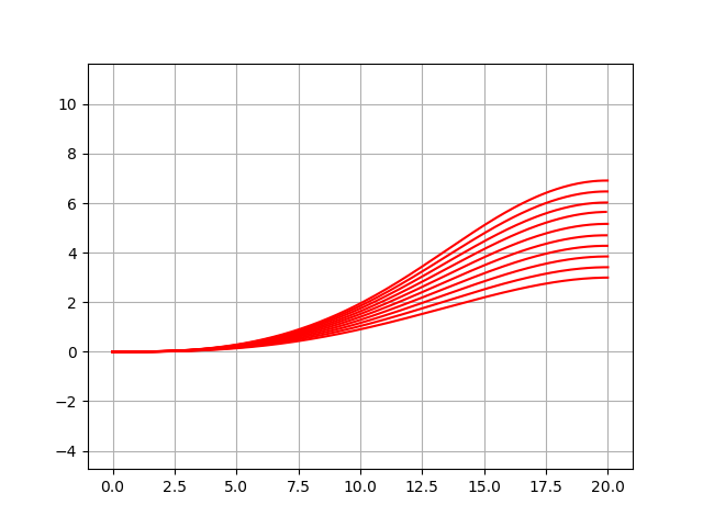
最终的结果是

2.4 state_lattice_planner.py

这部分主要实现论文《State Space Sampling of Feasible Motions for High-Performance Mobile Robot Navigation in Complex Environments》中状态空间采样算法

search_nearest_one_from_lookuptable(tx, ty, tyaw, lookup_table):同lookuptable_generator中方法
generate_path(target_states, k0):为target_states中采样得到的边界状态生成路径
calc_uniform_polar_states(nxy, nh, d, a_min, a_max, p_min, p_max)：根据状态空间采样参数进行均匀采样，返回采样得到的边界状态
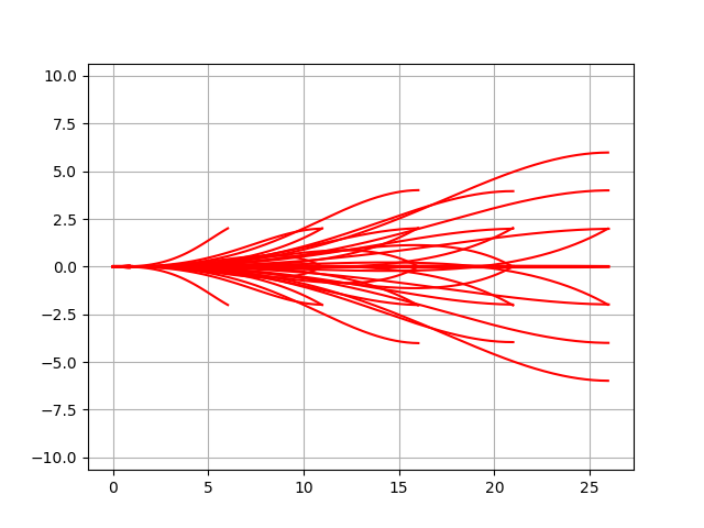
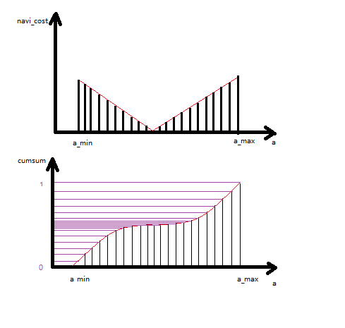
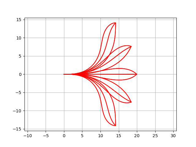
calc_biased_polar_states(goal_angle, ns, nxy, nh, d, a_min, a_max, p_min, p_max)：参考global guidance进行偏置采样，即cost高稀疏采样，cost低稠密采样。用采样位置点的角度和终点位置的角度之差代表cost。
- 在navigation function上均匀采样，离目标近时cost低，离目标远时cost高
- normalize，生成新的分布，离目标近时cnav结果也小；相反离目标远时cnav结果大
- 对分布进行积分，离目标近时，积分函数的变化缓慢；离目标远时，积分函数变化快
- 对积分结果csumnav 按照nxy个数均匀采样，在离目标近的区域由于积分函数变化缓慢，采样结果更为密集
calc_lane_states(l_center, l_heading, l_width, v_width, d, nxy)；车道线的采样
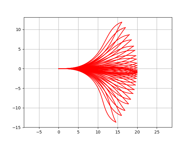
uniform_terminal_state_sampling_test1() 使用不同参数进行均匀采样

"""

State lattice planner with model predictive trajectory generator

author: Atsushi Sakai (@Atsushi_twi)

- lookuptable.csv is generated with this script: https://github.com/AtsushiSakai/PythonRobotics/blob/master/PathPlanning/ModelPredictiveTrajectoryGenerator/lookuptable_generator.py

Ref:

- State Space Sampling of Feasible Motions for High-Performance Mobile Robot Navigation in Complex Environments http://citeseerx.ist.psu.edu/viewdoc/download?doi=10.1.1.187.8210&rep=rep1&type=pdf

"""
import sys
import os
from matplotlib import pyplot as plt
import numpy as np
import math
import pandas as pd

sys.path.append(os.path.dirname(os.path.abspath(__file__))
                + "/../ModelPredictiveTrajectoryGenerator/")


try:
    import model_predictive_trajectory_generator as planner
    import motion_model
except ImportError:
    raise


table_path = os.path.dirname(os.path.abspath(__file__)) + "/lookuptable.csv"

show_animation = True


def search_nearest_one_from_lookuptable(tx, ty, tyaw, lookup_table):
    mind = float("inf")
    minid = -1

    for (i, table) in enumerate(lookup_table):

        dx = tx - table[0]
        dy = ty - table[1]
        dyaw = tyaw - table[2]
        d = math.sqrt(dx ** 2 + dy ** 2 + dyaw ** 2)
        if d <= mind:
            minid = i
            mind = d

    return lookup_table[minid]


def get_lookup_table():
    data = pd.read_csv(table_path)

    return np.array(data)


def generate_path(target_states, k0):
	"""
    k0是初始曲率，为target_states中的边界状态生成路径
    返回所有的路径和最优参数
    """
    # x, y, yaw, s, km, kf
    lookup_table = get_lookup_table()
    result = []

    for state in target_states:
        #从lookup table中找到最佳的参考参数
        bestp = search_nearest_one_from_lookuptable(
            state[0], state[1], state[2], lookup_table)

        target = motion_model.State(x=state[0], y=state[1], yaw=state[2])
        # 把最佳参考作为初始化参数
        init_p = np.array(
            [math.sqrt(state[0] ** 2 + state[1] ** 2), bestp[4], bestp[5]]).reshape(3, 1)
        # 优化路径，生成路径上点，及优化后参数p
        x, y, yaw, p = planner.optimize_trajectory(target, k0, init_p)
        # 把结果加入result
        if x is not None:
            print("find good path")
            result.append(
                [x[-1], y[-1], yaw[-1], float(p[0]), float(p[1]), float(p[2])])

    print("finish path generation")
    return result


def calc_uniform_polar_states(nxy, nh, d, a_min, a_max, p_min, p_max):
    """
    calc uniform state

    :param nxy: number of position sampling
    :param nh: number of heading sampleing
    :param d: distance of terminal state
    :param a_min: position sampling min angle
    :param a_max: position sampling max angle
    :param p_min: heading sampling min angle
    :param p_max: heading sampling max angle
    :return: states list
    """
    # 均匀的采样角度，计算位置
    angle_samples = [i / (nxy - 1) for i in range(nxy)]
    states = sample_states(angle_samples, a_min, a_max, d, p_max, p_min, nh)

    return states


def calc_biased_polar_states(goal_angle, ns, nxy, nh, d, a_min, a_max, p_min, p_max):
    """
    calc biased state，cost越小，采样越密集，cost越大，采样越稀疏

    :param goal_angle: goal orientation for biased sampling
    :param ns: number of biased sampling
    :param nxy: number of position sampling
    :param nxy: number of position sampling
    :param nh: number of heading sampleing
    :param d: distance of terminal state
    :param a_min: position sampling min angle
    :param a_max: position sampling max angle
    :param p_min: heading sampling min angle
    :param p_max: heading sampling max angle
    :return: states list
    """
	#位置角度按照ns个数均匀采样
    asi = [a_min + (a_max - a_min) * i / (ns - 1) for i in range(ns - 1)]
    # 计算cost，相当于对导航函数采样
    cnav = [math.pi - abs(i - goal_angle) for i in asi]
	# cost的总和
    cnav_sum = sum(cnav)
    cnav_max = max(cnav)

    # normalize，生成新的分布，位置角度与终点角度相差小时cnav结果也小；相反角度相差大时cnav结果也大
    cnav = [(cnav_max - cnav[i]) / (cnav_max * ns - cnav_sum)
            for i in range(ns - 1)]
	# 对分布进行积分，这里角度相差小时，积分函数的变化缓慢；角度相差大时，积分函数变化快
    csumnav = np.cumsum(cnav)
    di = []
    li = 0
    # 对积分结果csumnav 按照nxy个数均匀采样，这样在角度相差小的区域，由于积分函数变化缓慢，采样的结果会更为密集
    for i in range(nxy):
        for ii in range(li, ns - 1):
            if ii / ns >= i / (nxy - 1):
                di.append(csumnav[ii])
                li = ii - 1
                break

    states = sample_states(di, a_min, a_max, d, p_max, p_min, nh)

    return states


def calc_lane_states(l_center, l_heading, l_width, v_width, d, nxy):
    """

    calc lane states

    :param l_center: lane lateral position
    :param l_heading:  lane heading
    :param l_width:  lane width
    :param v_width: vehicle width
    :param d: longitudinal position
    :param nxy: sampling number
    :return: state list
    """
    xc = d
    yc = l_center

    states = []
    for i in range(nxy):
        delta = -0.5 * (l_width - v_width) + \
            (l_width - v_width) * i / (nxy - 1)
        xf = xc - delta * math.sin(l_heading)
        yf = yc + delta * math.cos(l_heading)
        yawf = l_heading
        states.append([xf, yf, yawf])

    return states


def sample_states(angle_samples, a_min, a_max, d, p_max, p_min, nh):
    states = []
    for i in angle_samples:
        #角度采样
        a = a_min + (a_max - a_min) * i
		#生成位置坐标
        for j in range(nh):
            xf = d * math.cos(a)
            yf = d * math.sin(a)
            #航向角
            if nh == 1:
                yawf = (p_max - p_min) / 2 + a
            else:
                yawf = p_min + (p_max - p_min) * j / (nh - 1) + a
            states.append([xf, yf, yawf])

    return states


def uniform_terminal_state_sampling_test1():
    #初始角速度
    k0 = 0.0
    #位置的采样数目
    nxy = 5
    #航向角采样数目
    nh = 3
   # 距离，采样位置
    d = 20
    # 位置分布的角度范围
    a_min = - np.deg2rad(45.0)
    a_max = np.deg2rad(45.0)
    # 航向角的范围
    p_min = - np.deg2rad(45.0)
    p_max = np.deg2rad(45.0)
    #均匀采样
    states = calc_uniform_polar_states(nxy, nh, d, a_min, a_max, p_min, p_max)
    result = generate_path(states, k0)

    for table in result:
        xc, yc, yawc = motion_model.generate_trajectory(
            table[3], table[4], table[5], k0)

        if show_animation:
            plt.plot(xc, yc, "-r")

    if show_animation:
        plt.grid(True)
        plt.axis("equal")
        plt.show()

    print("Done")


def uniform_terminal_state_sampling_test2():
    k0 = 0.1
    nxy = 6
    nh = 3
    d = 20
    a_min = - np.deg2rad(-10.0)
    a_max = np.deg2rad(45.0)
    p_min = - np.deg2rad(20.0)
    p_max = np.deg2rad(20.0)
    states = calc_uniform_polar_states(nxy, nh, d, a_min, a_max, p_min, p_max)
    result = generate_path(states, k0)

    for table in result:
        xc, yc, yawc = motion_model.generate_trajectory(
            table[3], table[4], table[5], k0)

        if show_animation:
            plt.plot(xc, yc, "-r")

    if show_animation:
        plt.grid(True)
        plt.axis("equal")
        plt.show()

    print("Done")


def biased_terminal_state_sampling_test1():
    k0 = 0.0
    nxy = 30
    nh = 2
    d = 20
    a_min = np.deg2rad(-45.0)
    a_max = np.deg2rad(45.0)
    p_min = - np.deg2rad(20.0)
    p_max = np.deg2rad(20.0)
    ns = 100
    goal_angle = np.deg2rad(0.0)
    states = calc_biased_polar_states(
        goal_angle, ns, nxy, nh, d, a_min, a_max, p_min, p_max)
    result = generate_path(states, k0)

    for table in result:
        xc, yc, yawc = motion_model.generate_trajectory(
            table[3], table[4], table[5], k0)
        if show_animation:
            plt.plot(xc, yc, "-r")

    if show_animation:
        plt.grid(True)
        plt.axis("equal")
        plt.show()


def biased_terminal_state_sampling_test2():
    k0 = 0.0
    nxy = 30
    nh = 1
    d = 20
    a_min = np.deg2rad(0.0)
    a_max = np.deg2rad(45.0)
    p_min = - np.deg2rad(20.0)
    p_max = np.deg2rad(20.0)
    ns = 100
    goal_angle = np.deg2rad(30.0)
    states = calc_biased_polar_states(
        goal_angle, ns, nxy, nh, d, a_min, a_max, p_min, p_max)
    result = generate_path(states, k0)

    for table in result:
        xc, yc, yawc = motion_model.generate_trajectory(
            table[3], table[4], table[5], k0)

        if show_animation:
            plt.plot(xc, yc, "-r")

    if show_animation:
        plt.grid(True)
        plt.axis("equal")
        plt.show()


def lane_state_sampling_test1():
    k0 = 0.0

    l_center = 10.0
    l_heading = np.deg2rad(0.0)
    l_width = 3.0
    v_width = 1.0
    d = 10
    nxy = 5
    states = calc_lane_states(l_center, l_heading, l_width, v_width, d, nxy)
    result = generate_path(states, k0)

    if show_animation:
        plt.close("all")

    for table in result:
        xc, yc, yawc = motion_model.generate_trajectory(
            table[3], table[4], table[5], k0)

        if show_animation:
            plt.plot(xc, yc, "-r")

    if show_animation:
        plt.grid(True)
        plt.axis("equal")
        plt.show()


def main():
    planner.show_animation = show_animation
    uniform_terminal_state_sampling_test1()
    uniform_terminal_state_sampling_test2()
    biased_terminal_state_sampling_test1()
    biased_terminal_state_sampling_test2()
    lane_state_sampling_test1()


if __name__ == '__main__':
    main()

均匀采样举例

有global guidance 的稠密稀疏采样

车道采样

ErinLiu虎哥的铲屎员

关注

11
点赞
踩
35

收藏

觉得还不错? 一键收藏
4
评论
读PythonRobotics StateLatticePlanner源码-代码注释篇

文章目录2.注释2.1motion_model.py2.2model_predictive_trajectory_generator.py2.3 lookuptable_generator.py2.4 state_lattice_planner.py接上篇读PythonRobotics StateLatticePlanner源码-原理篇2.注释2.1motion_model.py这部分主要定义state类型[x,y,yaw,v][x,y,yaw,v][x,y,yaw,v]，位置，航向，和速度。涉
复制链接

扫一扫