应用SVM预测澳大利亚降雨（含数据预处理与调参）

0 声明 

本文主要内容来自视频'【2020机器学习全集】菜菜的sklearn完整版，价值4999元的最全机器学习sklearn全集，赶紧收藏_哔哩哔哩_bilibili'，课件来自“https://pan.baidu.com/s/1Xl4o0PMA5ysUILeCKvm_2w，提取码：a967”。

本人只是在上述视频和课件的基础上进行了少许改动。

本文所用数据可以在“https://pan.baidu.com/s/1Xl4o0PMA5ysUILeCKvm_2w，提取码：a967”下载，也可以从'https://download.csdn.net/download/liuqihang11/21761805'直接获取。

1 数据预处理

1.1 导入数据

导入数据部分需要做的工作是以dataframe格式导入数据（潘大师的格式）；将标签与特征矩阵分开；查看特征矩阵各个特征的空缺值所占比例（这会影响到数据处理方式的选择）、各个特征以及标签的数据类型（连续型、离散型还是时间，这也会影响到缺省值处理以及数据编码），最后还需要检查是否存在标签不平衡问题（可能会需要平衡标签）

import pandas as pd
import numpy as np
from sklearn.model_selection import train_test_split

weather = pd.read_csv(r"weatherAUS5000.csv",index_col=0) # 以dataframe格式读取文件数据

# weather.head() # 查看数据
# 将特征矩阵和标签Y分开
X = weather.iloc[:, :-1]
Y = weather.iloc[:, -1]

# 探索特征类型（查看是否有空缺，空缺值占所有数据的比例情况，数据类型是什么）
X.info() 
X.isnull().mean()

# 探索标签类型，是否有空缺值
Y.isnull().sum()
np.unique(Y)

# 检测样本不均衡问题
Ytrain.value_counts()
Ytest.value_counts()

# 描述性统计查看是否有异常值
Xtrain.describe([0.01,0.05,0.1,0.25,0.5,0.75,0.9,0.99]).T
Xtest.describe([0.01,0.05,0.1,0.25,0.5,0.75,0.9,0.99]).T

1.2 划分测试集与训练集

在做数据处理之前就需要划分测试集与训练集，如果不这么做，可能会使得训练集与测试之间的信息相互混杂（例如采用均值或者众数填补空缺值），造成数据污染。

# 分训练集和测试集
Xtrain, Xtest, Ytrain, Ytest = train_test_split(X,Y,test_size=0.3,random_state=420) # 随机抽样

# 恢复索引
for i in [Xtrain, Xtest, Ytrain, Ytest]:
    i.index = range(i.shape[0])

1.3 将标签编码

二分类问题将标签替换为01编码

from sklearn.preprocessing import LabelEncoder 
encorder = LabelEncoder().fit(Ytrain) 

# 使用训练集进行训练，然后在训练集和测试集上分别进行transform
Ytrain = pd.DataFrame(encorder.transform(Ytrain))
Ytest = pd.DataFrame(encorder.transform(Ytest))

1.4 处理日期

日期本身对明天下雨与否是不产生影响的，但是今天是否下雨与明天是否下雨是有较强的相关关系的。注意到特征中有一个叫做“rainfall”，表示当前日期当前地区下的降雨量，换句话说，也就是”今
天的降雨量“，因此，可以将时间对气候的连续影响，转换为”今天是否下雨“这个特征，巧妙地将样本对应标签之间的联系，转换成是特征与标签之间的联系。

Xtrain["Rainfall"].head(20) # 查看rainfall的数据
Xtrain["Rainfall"].isnull().sum() # 查看是否有空值

Xtrain.loc[Xtrain.loc[:, "Rainfall"] >= 1, "RainToday"] = "Yes" # 大于1设置为下雨
Xtrain.loc[Xtrain.loc[:, "Rainfall"] < 1, "RainToday"] = "No" # 小于1设置为不下雨
Xtrain.loc[Xtrain.loc[:, "Rainfall"] == np.nan, "RainToday"] = np.nan # 空值还是为空

# 对test数据集执行同样的操作
Xtest.loc[Xtest["Rainfall"] >= 1,"RainToday"] = "Yes"
Xtest.loc[Xtest["Rainfall"] < 1,"RainToday"] = "No"
Xtest.loc[Xtest["Rainfall"] == np.nan,"RainToday"] = np.nan

按道理来说对于日期的处理到此结束，可以删除日期这一列了。然而又注意到降雨与否虽然与日期本身无关，但是却与当天所处的月份是有关的，根据生活常识，一年中某些月份的降雨量明显要多一些。因此，具体哪一天的日期没有用，但是月份却是有效的信息，应当予以保留。

Xtrain["Date"] = Xtrain["Date"].apply(lambda x:int(x.split("-")[1])) # 提取月份数字替换原来的日期

Xtrain = Xtrain.rename(columns={"Date":"Month"}) # 重命名date列为month

# 对test采取同样操作
Xtest["Date"] = Xtest["Date"].apply(lambda x:int(x.split("-")[1]))
Xtest = Xtest.rename(columns={"Date":"Month"})

1.5 处理地点值

地点显然与是否降雨有关的，与其说是地点，不如说是与地点所处的气候有关系。因此，需要将数据中的地点换为地点所对应的气候。然而注意到样本中的地点名称其实是气候站的名称，而气象站的名称可能是以当地小地点的名称命名的，这就比较麻烦，因为并不是所有的小地点都能够直接搜索到当地气候，一般而言，大城市是比较容易获取其气候信息的，但是好在所有的小地点都能够查询到地理位置的信息。那么问题就简单了，可以查询出大城市的气候信息与经纬度，再查出气象站的经纬度，找出离气象站最近的大城市，该大城市所对应的气候就是气象站的气候（这种方法可能不能保证完全正确，但大致来看还是没问题的）

cityll = pd.read_csv(r"cityll.csv",index_col=0) # 读取大城市的地理信息
city_climate = pd.read_csv(r"Cityclimate.csv") # 读取大城市的气候
samplecity = pd.read_csv(r"samplecity.csv",index_col=0) # 读取气象站的经纬度

# 查看读取的数据
city_climate.head()
cityll.head()
samplecity.head()

# 去掉度数符号
cityll["Latitudenum"] = cityll["Latitude"].apply(lambda x:float(x[:-1]))
cityll["Longitudenum"] = cityll["Longitude"].apply(lambda x:float(x[:-1]))
samplecity["Latitudenum"] = samplecity["Latitude"].apply(lambda x:float(x[:-1]))
samplecity["Longitudenum"] = samplecity["Longitude"].apply(lambda x:float(x[:-1]))

# 所有数据均为南维与东经，故不需要这两个信息
citylld = cityll.iloc[:,[0,5,6]]
samplecityd = samplecity.iloc[:,[0,5,6]]

#将city_climate中的气候添加到citylld中
citylld["climate"] = city_climate.iloc[:,-1]

#首先使用radians将角度转换成弧度
from math import radians, sin, cos, acos
citylld.loc[:,"slat"] = citylld.iloc[:,1].apply(lambda x : radians(x))
citylld.loc[:,"slon"] = citylld.iloc[:,2].apply(lambda x : radians(x))
samplecityd.loc[:,"elat"] = samplecityd.iloc[:,1].apply(lambda x : radians(x))
samplecityd.loc[:,"elon"] = samplecityd.iloc[:,2].apply(lambda x : radians(x))

import sys
# slat是起始地点的纬度，slon是起始地点的经度，elat是结束地点的纬度，elon是结束地点的经度
for i in range(samplecityd.shape[0]):
    slat = citylld.loc[:,"slat"]
    slon = citylld.loc[:,"slon"]
    elat = samplecityd.loc[i,"elat"]
    elon = samplecityd.loc[i,"elon"]
    dist = 6371.01 * np.arccos(np.sin(slat)*np.sin(elat) + 
                          np.cos(slat)*np.cos(elat)*np.cos(slon.values - elon))
    city_index = np.argsort(dist)[0]
    # 每次计算后，取距离最近的城市，然后将最近的城市和城市对应的气候都匹配到samplecityd中
    samplecityd.loc[i,"closest_city"] = citylld.loc[city_index,"City"]
    samplecityd.loc[i,"climate"] = citylld.loc[city_index,"climate"]

samplecityd.head(5) # 查看结果
# 确认无误后，取出样本城市所对应的气候，并保存
locafinal = samplecityd.iloc[:,[0,-1]]
locafinal.columns = ["Location","Climate"] # 给列重命名

# 设定locafinal的索引为地点
locafinal = locafinal.set_index(keys="Location")
# 气象站的名字替换成了对应的城市对应的气候，进行map匹配
Xtrain["Location"] = Xtrain["Location"].map(locafinal.iloc[:,0]) # 索引相同则替换为气候

# 城市的气候中所含的逗号和空格都去掉
Xtrain["Location"] = Xtrain["Location"].apply(lambda x:re.sub(",","",x.strip()))
Xtest["Location"] = Xtest["Location"].map(locafinal.iloc[:,0]).apply(lambda x:re.sub(",","",x.strip()))

修改列名
Xtrain = Xtrain.rename(columns={"Location":"Climate"})
Xtest = Xtest.rename(columns={"Location":"Climate"})

1.6 缺失值处理

一般而言，如果是分类型特征，则采用众数进行填补。如果是连续型特征，则采用均值来填补。另外，对于测试集中的空值，采用训练集的数据进行填补。因为在现实中，测试集未必是很多条数据，也许测试集只有一条数据，而某个特征上是空值，此时此刻测试集本身的众数根本不存在，为了避免这种尴尬的情况发生，假设测试集和训练集的数据分布和性质都是相似的，因此统一使用训练集的众数和均值来对测试集进行填补。

1.6.1 填补分类型数据并编码

#首先找出，分类型特征都有哪些
cate = Xtrain.columns[Xtrain.dtypes == "object"].tolist()
# 除了特征类型为"object"的特征，还有虽然用数字表示，但是本质为分类型特征的云层遮蔽程度
cloud = ["Cloud9am","Cloud3pm"]
cate = cate + cloud

# 对于分类型特征，使用众数来进行填补
from sklearn.impute import SimpleImputer #0.20, conda, pip

si = SimpleImputer(missing_values=np.nan,strategy="most_frequent")
# 注意，使用训练集数据来训练填补器，本质是在生成训练集中的众数
si.fit(Xtrain.loc[:,cate])

# 然后用训练集中的众数来同时填补训练集和测试集
Xtrain.loc[:,cate] = si.transform(Xtrain.loc[:,cate])
Xtest.loc[:,cate] = si.transform(Xtest.loc[:,cate])

# 将所有的分类型变量编码为数字，一个类别是一个数字
from sklearn.preprocessing import OrdinalEncoder #只允许二维以上的数据进行输入
oe = OrdinalEncoder()
# 利用训练集进行fit
oe = oe.fit(Xtrain.loc[:,cate])

# 用训练集的编码结果来编码训练和测试特征矩阵
Xtrain.loc[:,cate] = oe.transform(Xtrain.loc[:,cate])
Xtest.loc[:,cate] = oe.transform(Xtest.loc[:,cate])

Xtrain.loc[:,cate].head() # 查看编码效果
Xtest.loc[:,cate].head()

1.6.2 填补连续型数据

# 找出剩下的数值型数据
col = Xtrain.columns.tolist()
for i in cate:
    col.remove(i)

# 实例化模型，填补策略为"mean"表示均值
impmean = SimpleImputer(missing_values=np.nan,strategy = "mean")
# 用训练集来fit模型
impmean = impmean.fit(Xtrain.loc[:,col])
# 分别在训练集和测试集上进行均值填补
Xtrain.loc[:,col] = impmean.transform(Xtrain.loc[:,col])
Xtest.loc[:,col] = impmean.transform(Xtest.loc[:,col])

Xtest.isnull().mean() # 查看是否填补完成
Xtrain.isnull().mean()

1.7 数据无量纲化

SVM算法本质是计算距离，因此对于数据的量纲比较敏感，故需要对连续型数据无量纲化，注意，对于分类型数据，不进行无量纲化。一个特例是月份，虽然是数值型数据，也不需要无量纲化。

col.remove("Month")
from sklearn.preprocessing import StandardScaler # 数据转换为均值为0，方差为1的数据（分布不变）
ss = StandardScaler()
ss = ss.fit(Xtrain.loc[:,col])

Xtrain.loc[:,col] = ss.transform(Xtrain.loc[:,col])
Xtest.loc[:,col] = ss.transform(Xtest.loc[:,col])

Xtrain.head() # 查看标准化后的结果
Xtest.head()

到此为止数据的预处理结束。这一步之后，执行运算之前，最好保存一些处理好的数据。

Ytrain.to_csv("Ytrain.csv")
Xtrain.to_csv("Xtrain.csv")
Xtest.to_csv("Xtest.csv")
Ytest.to_csv("Ytest.csv")

2  基于sklearn建立SVM模型

from sklearn.svm import SVC
from sklearn.model_selection import cross_val_score
from sklearn.metrics import roc_auc_score, recall_score

Ytrain = Ytrain.iloc[:,0].ravel()
Ytest = Ytest.iloc[:,0].ravel()

#同时观察，精确性，recall以及AUC分数

for kernel in ["linear","poly","rbf","sigmoid"]:
    clf = SVC(kernel = kernel
              ,gamma="auto"
              ,degree = 1
              ,cache_size = 5000
             ).fit(Xtrain, Ytrain)
    result = clf.predict(Xtest)
    score = clf.score(Xtest,Ytest) # 返回accuracy
    recall = recall_score(Ytest, result) # 返回recall
    auc = roc_auc_score(Ytest,clf.decision_function(Xtest)) # 返回auc面积
    print("%s 's testing accuracy %f, recall is %f', auc is %f" % (kernel,score,recall,auc))
    print(datetime.datetime.fromtimestamp(time()-times).strftime("%M:%S:%f"))

linear 's testing accuracy 0.844000, recall is 0.469388', auc is 0.869029
00:05:063492
poly 's testing accuracy 0.840667, recall is 0.457726', auc is 0.868157
00:05:755614
rbf 's testing accuracy 0.813333, recall is 0.306122', auc is 0.814873
00:08:202100
sigmoid 's testing accuracy 0.655333, recall is 0.154519', auc is 0.437308
00:08:888237

3 调参

3.1 追求最高的recall

想要最高的recall，可以牺牲准确度，若想不计一切代价来捕获少数类，那首先可以打开class_weight参数，使用balanced模式来调节recall

for kernel in ["linear","poly","rbf","sigmoid"]:
    clf = SVC(kernel = kernel
              ,gamma="auto"
              ,degree = 1
              ,cache_size = 5000
              ,class_weight = "balanced" # 使用balanced均衡数据
             ).fit(Xtrain, Ytrain)
    result = clf.predict(Xtest)
    score = clf.score(Xtest,Ytest)
    recall = recall_score(Ytest, result)
    auc = roc_auc_score(Ytest,clf.decision_function(Xtest))
    print("%s 's testing accuracy %f, recall is %f', auc is %f" % (kernel,score,recall,auc))
    print(datetime.datetime.fromtimestamp(time()-times).strftime("%M:%S:%f"))

linear 's testing accuracy 0.796667, recall is 0.775510', auc is 0.870062
00:05:951088
poly 's testing accuracy 0.793333, recall is 0.763848', auc is 0.871448
00:06:982332
rbf 's testing accuracy 0.803333, recall is 0.600583', auc is 0.819713
00:09:927460
sigmoid 's testing accuracy 0.562000, recall is 0.282799', auc is 0.437119
00:11:631901

根据程序运行结果，linear核 的效果最好，然后可以将class_weight调节得更加倾向于少数类，来不计代价提升recall。

'''追求最高的recall'''
clf = SVC(kernel = "linear"
          ,gamma="auto"
          ,cache_size = 5000
          ,class_weight = {1:15} #注意，这里写的其实是，类别1：15，隐藏了类别0：1这个比例
         ).fit(Xtrain, Ytrain)
result = clf.predict(Xtest)
score = clf.score(Xtest,Ytest)
recall = recall_score(Ytest, result)
auc = roc_auc_score(Ytest,clf.decision_function(Xtest))
print("testing accuracy %f, recall is %f', auc is %f" %(score,recall,auc))
print(datetime.datetime.fromtimestamp(time()-times).strftime("%M:%S:%f"))

testing accuracy 0.548000, recall is 0.970845', auc is 0.867172
00:10:776214

3.2 追求最高的accuracy

要追求accuracy，首先要看一下样本的不均衡状况，如果样本非常不均衡，但是此时却有很多多数类被判错的话，那可以让模型任性地把所有地样本都判断为0，完全不顾少数类。可以使用混淆矩阵来计算我们的特异度，如果特异度非常高，则证明多数类上已经很难被操作了。

from sklearn.metrics import confusion_matrix as CM

clf = SVC(kernel = "linear"
          ,gamma="auto"
          ,cache_size = 5000
         ).fit(Xtrain, Ytrain)
result = clf.predict(Xtest)
cm = CM(Ytest,result,labels=(1,0))
specificity = cm[1,1]/cm[1,:].sum()

特异度结果显示为0.9550561797752809，以看到，特异度非常高，表示几乎所有的的0都被判断正确了，还有不少1也被判断正确了。此时如果要求模型将所有的类都判断为0，则已经被判断正确的少数类会被误伤，整体的准确率一定会下降。而如果希望通过让模型捕捉更多少数类来提升精确率的话，却无法实现，因为一旦让模型更加倾向于少数类，就会有更多的多数类被判错。

可以试试看使用class_weight向模型少数类的方向稍微调整，查看是否有更多的空间来提升的准确
率。如果在轻微向少数类方向调整过程中，出现了更高的准确率，则说明模型还没有到极限。

irange = np.linspace(0.01,0.05,10)

for i in irange:
    times = time()
    clf = SVC(kernel="linear", gamma="auto", cache_size=5000, class_weight={0:1,1:1+i}
              ).fit(Xtrain, Ytrain)
    result = clf.predict(Xtest)
    score = clf.score(Xtest, Ytest)
    recall = recall_score(Ytest, result)
    auc = roc_auc_score(Ytest, clf.decision_function(Xtest))
    print("under ratio 1:%f testing accuracy %f, recall is %f', auc is %f" %
          (1+i, score, recall, auc))
    print(datetime.datetime.fromtimestamp(time()-times).strftime("%M:%S:%f"))

under ratio 1:1.010000 testing accuracy 0.844667, recall is 0.475219', auc is 0.869157
00:05:502289
under ratio 1:1.014444 testing accuracy 0.844667, recall is 0.478134', auc is 0.869185
00:05:576092
under ratio 1:1.018889 testing accuracy 0.844000, recall is 0.478134', auc is 0.869228
00:05:851356
under ratio 1:1.023333 testing accuracy 0.845333, recall is 0.481050', auc is 0.869175
00:05:644908
under ratio 1:1.027778 testing accuracy 0.844000, recall is 0.481050', auc is 0.869394
00:05:842413
under ratio 1:1.032222 testing accuracy 0.844000, recall is 0.481050', auc is 0.869528
00:05:256941
under ratio 1:1.036667 testing accuracy 0.844000, recall is 0.481050', auc is 0.869659
00:05:473338
under ratio 1:1.041111 testing accuracy 0.844667, recall is 0.483965', auc is 0.869629
00:05:087399
under ratio 1:1.045556 testing accuracy 0.844667, recall is 0.483965', auc is 0.869712
00:05:103354
under ratio 1:1.050000 testing accuracy 0.845333, recall is 0.486880', auc is 0.869863
00:05:106347

根据结果显示0.844667的accuracy已经是极限了。要想进一步提升模型的准确率，调参不能满足要求，剩下能做的就是更换算法了。下面使用逻辑回归做一次尝试。

from sklearn.linear_model import LogisticRegression as LR # svm到极限了，换个模型

C_range = np.linspace(5,10,10)
for C in C_range:
    logclf = LR(solver="liblinear",C=C).fit(Xtrain, Ytrain)
    print(C,logclf.score(Xtest,Ytest))

5.0 0.8493333333333334
5.555555555555555 0.8493333333333334
6.111111111111111 0.8486666666666667
6.666666666666667 0.8493333333333334
7.222222222222222 0.8493333333333334
7.777777777777778 0.8493333333333334
8.333333333333334 0.8493333333333334
8.88888888888889 0.8493333333333334
9.444444444444445 0.8493333333333334
10.0 0.8493333333333334

使用逻辑回归的效果明显优于SVM，但是还是没有实现一个比较大的提升。要将模型的精确度提
升到90%以上，也许需要集成算法：比如，梯度提升树等。

3.3 追求accuracy与recall之间的平衡

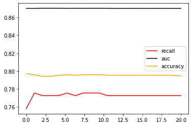
尝试调节C值来看看效果。

import matplotlib.pyplot as plt
'''追求平衡recall与accuracy的平衡'''
C_range = np.linspace(0.01, 20, 20) # 选出最优的C值,C越大，运行时间越长
recallall = []
aucall = []
scoreall = []
for C in C_range:
    times = time()
    clf = SVC(kernel="linear", C=C, cache_size=5000, class_weight="balanced"
              ).fit(Xtrain, Ytrain)
    result = clf.predict(Xtest)
    score = clf.score(Xtest, Ytest)
    recall = recall_score(Ytest, result)
    auc = roc_auc_score(Ytest, clf.decision_function(Xtest))
    recallall.append(recall)
    aucall.append(auc)
    scoreall.append(score)
print(max(aucall), C_range[aucall.index(max(aucall))])
plt.figure()
plt.plot(C_range, recallall, c="red", label="recall")
plt.plot(C_range, aucall, c="black", label="auc")
plt.plot(C_range, scoreall, c="orange", label="accuracy")
plt.legend()
plt.show() # 最终确定c为3.162105263157895

0.8701704166047206 3.162105263157895

把目前为止最佳的C值3.162105263157895带入模型，看看准确率，Recall的具体值：

'''追求平衡recall与accuracy的平衡'''
clf = SVC(kernel = "linear",C=3.162105263157895,cache_size = 5000
          ,class_weight = "balanced"
         ).fit(Xtrain, Ytrain)
result = clf.predict(Xtest)
score = clf.score(Xtest,Ytest)
recall = recall_score(Ytest, result)
auc = roc_auc_score(Ytest,clf.decision_function(Xtest))
print("testing accuracy %f,recall is %f', auc is %f" % (score,recall,auc))

testing accuracy 0.794000,recall is 0.772595', auc is 0.870170

可以看到，这种情况下模型的准确率，Recall和AUC都没有太差，但是也没有太好，这也许就是模型平衡后的一种结果。现在，光是调整支持向量机本身的参数，已经不能够满足我们的需求了，要想让AUC面积更进一步，需要绘制ROC曲线，查看是否可以通过调整阈值来对这个模型进行改进。

from sklearn.metrics import roc_curve as ROC # 通过ROC曲线确定最佳阈值
import matplotlib.pyplot as plt
from sklearn.metrics import accuracy_score as AC

FPR, Recall, thresholds = ROC(Ytest,clf.decision_function(Xtest),pos_label=1) # pos_label为感兴趣的标签，1为少数类
area = roc_auc_score(Ytest,clf.decision_function(Xtest))
print(area)

plt.figure()
plt.plot(FPR, Recall, color='red',
         label='ROC curve (area = %0.2f)' % area)
plt.plot([0, 1], [0, 1], color='black', linestyle='--')
plt.xlim([-0.05, 1.05])
plt.ylim([-0.05, 1.05])
plt.xlabel('False Positive Rate')
plt.ylabel('Recall')
plt.title('Receiver operating characteristic example')
plt.legend(loc="lower right")
plt.show()

maxindex = (Recall - FPR).tolist().index(max(Recall - FPR)) # 计算最优阈值索引
clf = SVC(kernel = "linear",C=3.1663157894736838,cache_size = 5000
          ,class_weight = "balanced"
         ).fit(Xtrain, Ytrain)
prob = pd.DataFrame(clf.decision_function(Xtest)) # 返回距离
prob.loc[prob.iloc[:,0] >= thresholds[maxindex],"y_pred"]=1 # 手动设置分类
prob.loc[prob.iloc[:,0] < thresholds[maxindex],"y_pred"]=0
score = AC(Ytest,prob.loc[:,"y_pred"].values) # 计算准确率
recall = recall_score(Ytest, prob.loc[:,"y_pred"]) # 计算召回率
print("testing accuracy %f,recall is %f" % (score,recall))
print(datetime.datetime.fromtimestamp(time()-times).strftime("%M:%S:%f"))

0.8701603372550402
testing accuracy 0.789333,recall is 0.804665

4 小结

到此为止，利用SVM算法进行天气预测的模型构建过程就已经完成了 。总共经历了数据预处理、模型搭建以及调参三个过程。

数据预处理包括测试集与训练集数据划分、查看数据的缺失值或者异常值、处理困难特征（地点、日期等）、特征分类（连续型、离散型）、采用不同方法对不同类型的数据进行缺失填补、连续型数字无量纲化等。

模型搭建包括选择合适的模型算法（这里选择的是SVM算法）与模型评估参数的选择（accuracy、recall、auc面积等等）。

调参是一个比较复杂的问题，需要根据不同的任务目标选取调参方向。本例给出了三个调参方向，第一个是只考虑最高的recall值，可以通过调整class_weight参数来实现最高的recall；第二个是考虑最高的accuracy，也可以试试向少数类样本方向调节class_weight，或者换用一些集成算法；最后一个是追求accuracy与recall之间的平衡，可以试试调节核函数的C参数以及绘制出ROC曲线选定最佳的阈值试试效果。

如果采用了各种调参手段效果均不太理想，可以考虑更改算法或者采用其他的方法进行数据预处理。

5 完整代码

这里不放完整代码，直接将上述代码复制到juopyter notebook中分段运行效果更好。