PointNet、PointNet++

最新推荐文章于 2024-06-02 23:40:08 发布

nuttee

最新推荐文章于 2024-06-02 23:40:08 发布

阅读量3k

点赞数 1

分类专栏：计算机理论文章标签： Point Segementation 3D PointNet

本文链接：https://blog.csdn.net/lrwwll/article/details/88709616

版权

计算机理论专栏收录该内容

16 篇文章 1 订阅

订阅专栏

PointNet

PointNet vanilla

亮点

端到端学习
通用的框架
- Object Classification
- Object Part Segmentation
- Semantic Scene Parsing

Challenges

输入的点云是无序的
需要做到对几何变换的invariance

C1:
作为输入的点云实际上就是point的集合，是无序的，但是目前的深度学习关注的还是一些regular input representation的，比如sequences, images, volumes，在之前的点云研究中，都是先将点云处理转化为其他的表示形式，然后再作为输入送入深度神经网络中，这实际上损失了一些信息。作者希望能够直接将点云集合作为输入送入神经网络，完成端到端的学习。

而要达到这个目的，就要做到模型对点云集合作为输入的顺序做到‘免疫’。

这个问题可以使用对称函数解决，直观地说，如果一个函数的输出与输入的顺序无关，那么就说这个函数是一个对称函数，比较常见的像：加法、最大值函数等。

这里h作者使用了多层感知机来提取点特征，但是在实际的implementation里用的还是1*1 convolution，g使用的是max pooling这个对称函数来最终得到全局特征，理论上f可以拟合任意的连续对称函数，但是数学证明我并没有看太懂。在经过f的作用之后，便得到了点云的全局特征，在分类任务上已经可以直接使用了，但是对于点云分割来说，还需要局部特征与全局特征进行融合。作者直接将习得的全局特征与之前习得的点特征进行串联，在此基础上，进一步提取点特征。

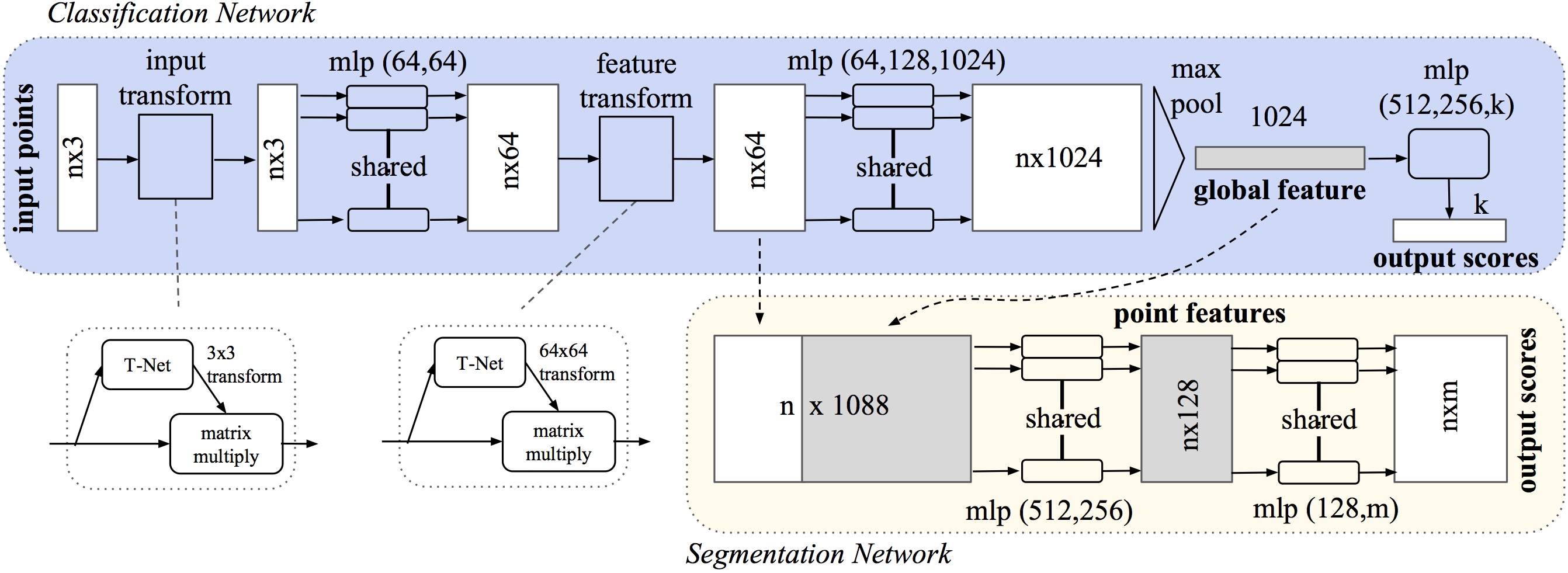
下面便是进行分类任务的代码，对应了网络架构图中点云输入通过一个input transform得到的nx3之后的网络：

def get_model(point_cloud, is_training, bn_decay=None):
    """ Classification PointNet, input is BxNx3, output Bx40 """
    batch_size = point_cloud.get_shape()[0].value
    num_point = point_cloud.get_shape()[1].value
    end_points = {}
    input_image = tf.expand_dims(point_cloud, -1)
    
    # Point functions (MLP implemented as conv2d)
    net = tf_util.conv2d(input_image, 64, [1,3],
                         padding='VALID', stride=[1,1],
                         bn=True, is_training=is_training,
                         scope='conv1', bn_decay=bn_decay)
    net = tf_util.conv2d(net, 64, [1,1],
                         padding='VALID', stride=[1,1],
                         bn=True, is_training=is_training,
                         scope='conv2', bn_decay=bn_decay)
    net = tf_util.conv2d(net, 64, [1,1],
                         padding='VALID', stride=[1,1],
                         bn=True, is_training=is_training,
                         scope='conv3', bn_decay=bn_decay)
    net = tf_util.conv2d(net, 128, [1,1],
                         padding='VALID', stride=[1,1],
                         bn=True, is_training=is_training,
                         scope='conv4', bn_decay=bn_decay)
    net = tf_util.conv2d(net, 1024, [1,1],
                         padding='VALID', stride=[1,1],
                         bn=True, is_training=is_training,
                         scope='conv5', bn_decay=bn_decay)

    # Symmetric function: max pooling
    net = tf_util.max_pool2d(net, [num_point,1],
                             padding='VALID', scope='maxpool')
    
    # MLP on global point cloud vector
    net = tf.reshape(net, [batch_size, -1])
    net = tf_util.fully_connected(net, 512, bn=True, is_training=is_training,
                                  scope='fc1', bn_decay=bn_decay)
    net = tf_util.fully_connected(net, 256, bn=True, is_training=is_training,
                                  scope='fc2', bn_decay=bn_decay)
    net = tf_util.dropout(net, keep_prob=0.7, is_training=is_training,
                          scope='dp1')
    net = tf_util.fully_connected(net, 40, activation_fn=None, scope='fc3')

    return net, end_points

C2:

为了不受几何变换，比如刚性变换的影响，作者借鉴了STN，但是采用了比之更加简单的方法：使用一个小型的神经网络T-Net去预测一个仿射变换矩阵，然后直接将输入与这个矩阵相乘。
T-net1
T-net2

下面是T-Net的具体实现，第一个net对应的是论文中网络架构图中的input transform，第二个net对应的是论文中的feature transform，输入不同，网络结构和参数自然有一些变化。

def input_transform_net(point_cloud, is_training, bn_decay=None, K=3):
    """ Input (XYZ) Transform Net, input is BxNx3 gray image
        Return:
            Transformation matrix of size 3xK """
    batch_size = point_cloud.get_shape()[0].value
    num_point = point_cloud.get_shape()[1].value

    input_image = tf.expand_dims(point_cloud, -1)
    net = tf_util.conv2d(input_image, 64, [1,3],
                         padding='VALID', stride=[1,1],
                         bn=True, is_training=is_training,
                         scope='tconv1', bn_decay=bn_decay)
    net = tf_util.conv2d(net, 128, [1,1],
                         padding='VALID', stride=[1,1],
                         bn=True, is_training=is_training,
                         scope='tconv2', bn_decay=bn_decay)
    net = tf_util.conv2d(net, 1024, [1,1],
                         padding='VALID', stride=[1,1],
                         bn=True, is_training=is_training,
                         scope='tconv3', bn_decay=bn_decay)
    net = tf_util.max_pool2d(net, [num_point,1],
                             padding='VALID', scope='tmaxpool')

    net = tf.reshape(net, [batch_size, -1])
    net = tf_util.fully_connected(net, 512, bn=True, is_training=is_training,
                                  scope='tfc1', bn_decay=bn_decay)
    net = tf_util.fully_connected(net, 256, bn=True, is_training=is_training,
                                  scope='tfc2', bn_decay=bn_decay)

    with tf.variable_scope('transform_XYZ') as sc:
        assert(K==3)
        weights = tf.get_variable('weights', [256, 3*K],
                                  initializer=tf.constant_initializer(0.0),
                                  dtype=tf.float32)
        biases = tf.get_variable('biases', [3*K],
                                 initializer=tf.constant_initializer(0.0),
                                 dtype=tf.float32)
        biases += tf.constant([1,0,0,0,1,0,0,0,1], dtype=tf.float32)
        transform = tf.matmul(net, weights)
        transform = tf.nn.bias_add(transform, biases)

    transform = tf.reshape(transform, [batch_size, 3, K])
    return transform

def feature_transform_net(inputs, is_training, bn_decay=None, K=64):
    """ Feature Transform Net, input is BxNx1xK
        Return:
            Transformation matrix of size KxK """
    batch_size = inputs.get_shape()[0].value
    num_point = inputs.get_shape()[1].value

    net = tf_util.conv2d(inputs, 64, [1,1],
                         padding='VALID', stride=[1,1],
                         bn=True, is_training=is_training,
                         scope='tconv1', bn_decay=bn_decay)
    net = tf_util.conv2d(net, 128, [1,1],
                         padding='VALID', stride=[1,1],
                         bn=True, is_training=is_training,
                         scope='tconv2', bn_decay=bn_decay)
    net = tf_util.conv2d(net, 1024, [1,1],
                         padding='VALID', stride=[1,1],
                         bn=True, is_training=is_training,
                         scope='tconv3', bn_decay=bn_decay)
    net = tf_util.max_pool2d(net, [num_point,1],
                             padding='VALID', scope='tmaxpool')

    net = tf.reshape(net, [batch_size, -1])
    net = tf_util.fully_connected(net, 512, bn=True, is_training=is_training,
                                  scope='tfc1', bn_decay=bn_decay)
    net = tf_util.fully_connected(net, 256, bn=True, is_training=is_training,
                                  scope='tfc2', bn_decay=bn_decay)

    with tf.variable_scope('transform_feat') as sc:
        weights = tf.get_variable('weights', [256, K*K],
                                  initializer=tf.constant_initializer(0.0),
                                  dtype=tf.float32)
        biases = tf.get_variable('biases', [K*K],
                                 initializer=tf.constant_initializer(0.0),
                                 dtype=tf.float32)
        biases += tf.constant(np.eye(K).flatten(), dtype=tf.float32)
        transform = tf.matmul(net, weights)
        transform = tf.nn.bias_add(transform, biases)

    transform = tf.reshape(transform, [batch_size, K, K])
    return transform

PointNet++

PointNet++主要就是对PointNet的改进。由于PointNet不能很好地捕捉由度量空间引入的局部结构，也就限制了它识别细粒度类别的能力和对复杂场景的泛化能力。

PointNet的基本思想是对输入点云中的每一个点学习其对应的空间编码，之后再利用所有点的特征得到一个全局的点云特征，这里欠缺了对局部特征的提取和处理，但是探究局部特征已经在CNN中被证明很重要，传统的二维CNN接受规则输入，并且在不同层捕获不同尺度的特征。

PointNet++的思路很简单：首先通过距离度量将点云集合划分成一些重叠的局部区域，然后从邻域内提取局部特征，然后从这些局部特征中提取出更高层的特征。这一过程会不断重复直到得到整个点云集合的全局特征。

PointNet++的分层模型由一系列的abstraction level组成，而abstraction level包括三个部分：Sampling layer, Grouping layer, PointNet layer。其中Sampling layer从输入的点云中选择出一个点集合，也就是那些局部区域的中心点；Grouping layer通过寻找中心点的邻近点组成局部区域；而PointNet则被用来提取特征。

Chanllenges

2 Hows

how to abstract sets of points or local features through a local feature learner
how to generate the partitioning of the point set

C1
很自然地，作者使用了PointNet作为特征提取的手段。

C2
如何进行点云划分？

点球模型 $\rightarrow$ 选中心点(Sampling layer)，选半径(Grouping layer)。

Sampling layer: 如何选中心点？使用FPS算法(Farthest Point Sampling)：先随机选择一个点，然后再选择离这个点最远的点作为起点，再继续迭代，直到选出全部需要的点为止。

Grouping layer: 如何选半径？这就牵扯到另外一个问题：密度适应。由于点云中密度并不是处处相等的，所以不能都设置为相同的半径，这样可能会因为有的中心点邻域内密度较小导致采样不到足够多的点而提取不到有用的特征。所以，作者提出了一种尺度（密度）适应的方法。

这里作者提出了两种方案：MSG(Multi-scale Gourping)和MRG(Multi-resolution layer)

一图胜千言，作者画的示意图很棒，能够让人很轻松地get到作者的意思。
MSR-MGR

MSR
简单粗暴地设置几个不同的尺度，分别在这些尺度下提取特征，然后将不同尺度的特征进行concat。但是不同尺度的融合作者也是有讲究的，对每个训练集的点，随机选择一个概率进行dropout，在测试时，使用所有的点。
MGR
MSR因为是对所有的中心点的领域进行不同尺度的特征提取，因此计算开销很大。MGR的提出就是为了缓和计算开销的问题。图b中左边灰色的vector是由subregion使用abstraction level得到的特征，右边是由所有的raw points得到的点特征。左边的可以看作是比较全局的部分，右边的可以看作是比较局部的部分，通过这两个部分的结合，能够比较好地控制全局和局部的关系。当区域密度比较小的时候，说明局域特征没有全局特征可靠，需要赋给全局特征一个较大的权重，反之亦然。

PointNet++

由PointNet++的网络结构可以看到，对于分类任务，和PointNet是一样的，但是分割任务就有些不同了。因为PointNet++在abstraction layers中，进行了点采样，但是segementation任务中需要所有的点。一种解决办法是在abstraction layers中，把点云中所有的点都作为中心点，但显然这是不切实际的。另一种方法是将下采样的点特征传播回原始的数据点。这里使用了类似于FCN的across level skip links，同时进行KNN插值(feature values)。先将高层的 $N_l$ 特征值插值到低层的 $N_{l-1}$ 相应坐标，然后再和set abstraction layer的特征进行串联，送到类似于1*1 convolutional的unit pointnet中，最后通过全连接层和relu来更新点特征。

$K N N$ 中的权重用的是： inverse distance weighted average based on k nearest neighbors

knn

nuttee

关注

1
点赞
踩
14

收藏

觉得还不错? 一键收藏
3
评论
PointNet、PointNet++

PointNetPointNet vanilla亮点端到端学习通用的框架Object ClassificationObject Part SegmentationSemantic Scene ParsingChallenges输入的点云是无序的需要做到对几何变换的invarianceC1:作为输入的点云实际上就是point的集合，是无序的，但是目前的深度学习关...
复制链接

扫一扫