logistic regression及其Python实现

1.(逻辑斯蒂分布)logistic distribution

X是连续型随机变量,则logistic distribution是:

$F(x)=P(X\le x)=\frac{1}{1+e^-(x-u)/\gamma } \space , \space f(x)=F'(x)=\frac{e^-(x-\mu)/\gamma}{\gamma(1+e^-(x-\mu)/\gamma)^2}$
$\mu是位置参数，\gamma是形状参数。$
其形状如下：

2.logistic 回归模型

• 一种分类模型，由条件概率分布P(Y|X)表示，是一种判别模型
• 逻辑回归模型的定义：
  
  • $P(Y=1|x)=\frac{exp(\omega x+b)}{1+exp(\omega x+b)}$
  • $P(Y=0|x)=\frac{1}{1+exp(\omega x+b)}$

3.模型参数的估计

对于给定的训练数据集， $T={(x_1,y_1),(x_2,y_2),...,(x_N,Y_N)} \space ,y_i\in \{0,1\}$,估计其参数的方法有,

3.1 极大似然估计

• 记，$P(Y=1|x)=\pi (x) \space ,\space P(Y=0|x)=1-\pi(x)$
• 那么模型的极大似然函数为：$\prod\limits_{i=1}^{N}[\pi(x_i)]^{y_i}[1-\pi(x_i)^{1-y_i}]$
• 模型的对数似然函数为：$L(\omega)=\sum\limits_{i=1}^N[y_ilog\pi(x_i)+(1-y_i)log(1-\pi(x_i))]$
• 求$L(\omega)$的极大值即可得到$\omega$的估计值。

3.2梯度下降法

• 损失函数：$J(\omega)=-\frac{1}{N}[\sum\limits_{i=1}^{N}y_ilogh_{\omega}(x_i)+(1-y_i)log(1-h_{\omega}(x_i))]$
• 梯度：$\frac{\partial J(\omega)}{\partial \omega_{j}}=\frac{\sum\limits_{i=1}^{N}(h_{\omega}(x_i)-y_i)x_i^j}{N}$
• 参数更新：$\omega_j:=\omega_j-\alpha\frac{\partial J(\omega)}{\partial(\omega_j)}$

4.Python 代码实现

使用的数据下载（终端）：wget https://raw.githubusercontent.com/lxrobot/General-source-code/master/logisticRegression/data.csv

#!/usr/bin/env python2
# -*- coding: utf-8 -*-
"""
Created on Tue Jul 24 14:54:18 2018
@author: rd
"""
from __future__ import division
import numpy as np
import matplotlib.pyplot as plt
from copy import deepcopy
import math

def loadData():
    tmp=np.loadtxt("data.csv",dtype=np.str,delimiter=",")
    data=tmp[1:,:].astype(np.float)
    np.random.shuffle(data)
    train_data=data[:int(0.7*len(data)),:]
    test_data=data[int(0.7*len(data)):,:]
    train_X=train_data[:,:-1]/50-1.0 #feature normalization[-1,1]
    train_Y=train_data[:,-1]
    test_X=test_data[:,:-1]/50-1.0
    test_Y=test_data[:,-1]
    return train_X,train_Y,test_X,test_Y

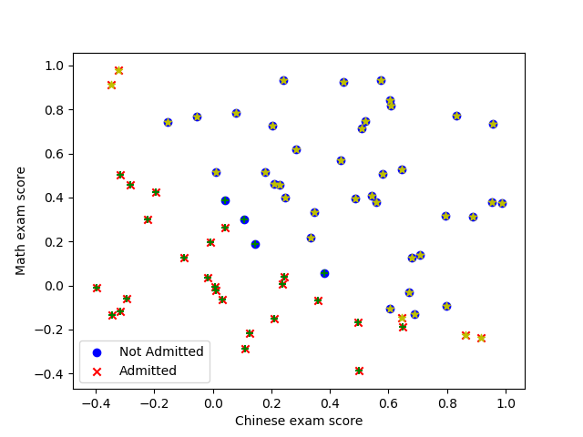
#pos=np.where(train_Y==1.0)
#neg=np.where(train_Y==0.0)
#plt.scatter(train_X[pos,0],train_X[pos,1],marker='o', c='b')
#plt.scatter(train_X[neg,0],train_X[neg,1],marker='x', c='r')
#plt.xlabel('Chinese exam score')
#plt.ylabel('Math exam score')
#plt.legend(['Not Admitted', 'Admitted'])
#plt.show()

#The sigmoid function
def sigmoid(z):
    return 1/(1+np.exp(-z))

def loss(h,Y):
    return (-Y*np.log(h)-(1-Y)*np.log(1-h)).mean()

def predict(X,theta,threshold):
    bias=np.ones((X.shape[0],1))
    X=np.concatenate((X,bias),axis=1)
    z=np.dot(X,theta)
    h=sigmoid(z)
    pred=(h>threshold).astype(float)
    return pred

def logisticRegression(X,Y,alpha,num_iters):
    model={}
    bias=np.ones((X.shape[0],1))
    X=np.concatenate((X,bias),axis=1)
    theta=np.ones(X.shape[1])
    for step in xrange(num_iters):
        z=np.dot(X,theta)
        h=sigmoid(z)
        grad=np.dot(X.T,(h-Y))/Y.size
        theta-=alpha*grad
        if step%1000==0:
            z=np.dot(X,theta)
            h=sigmoid(z)
            print "{} steps, loss is {}".format(step,loss(h,Y))
            print "accuracy is {}".format((predict(X[:,:-1],theta,0.5)==Y).mean()) 
    model={'theta':theta}
    return model

train_X,train_Y,test_X,test_Y=loadData()
model=logisticRegression(train_X,train_Y,alpha=0.01,num_iters=40000)
print "The test accuracy is {}".format((predict(test_X,model['theta'],0.5)==test_Y).mean())   

输出：

>>>python
0 steps, loss is 0.640056024601
accuracy is 0.614285714286
1000 steps, loss is 0.465700342681
accuracy is 0.757142857143
2000 steps, loss is 0.412992043943
accuracy is 0.885714285714
...
The test accuracy is 0.866666666667

预测结果：(黄色星号，绿色十字为预测值)

---

refer
[1] https://towardsdatascience.com/building-a-logistic-regression-in-python-step-by-step-becd4d56c9c8