Real-Time Rendering——9.8.1 Normal Distribution Functions正态分布函数

The normal distribution function has a significant effect on the appearance of the rendered surface. The shape of the NDF, as plotted on the sphere of microfacet normals, determines the width and shape of the cone of reflected rays (the specular lobe), which in turn determines the size and shape of specular highlights. The NDF affects the overall perception of surface roughness, as well as more subtle visual aspects such as whether highlights have a distinct edge or are surrounded by haze. 

正态分布函数对渲染表面的外观有重要影响。绘制在微法面法线球体上的NDF的形状决定了反射光线圆锥(镜面反射波瓣)的宽度和形状，进而决定了镜面反射高光的大小和形状。NDF影响表面粗糙度的整体感觉，以及更微妙的视觉方面，例如高光是否具有明显的边缘或被薄雾包围。

However, the specular lobe is not a simple copy of the NDF shape. It, and thus the highlight shape, is distorted to a greater or lesser degree depending on surface curvature and view angle. This distortion is especially strong for flat surfaces viewed at glancing angles, as shown in Figure 9.35. Ngan et al. [1271] present an analysis of the reason behind this distortion.

然而，镜面波瓣并不是NDF形状的简单复制。取决于表面曲率和视角，它以及因此高光形状会或多或少地变形。如图9.35所示，从掠射角观察平面时，这种变形特别强烈。Ngan等人[1271]对这种扭曲背后的原因进行了分析。

Figure 9.35. The images on the left are rendered with the non-physical Phong reflection model. This model’s specular lobe is rotationally symmetrical around the reflection vector. Such BRDFs were often used in the early days of computer graphics. The images in the center are rendered with a physically based microfacet BRDF. The top left and center show a planar surface lit at a glancing angle. The top left shows an incorrect round highlight, while the center displays the characteristic highlight elongation on the microfacet BRDF. This center view matches reality, as shown in the photographs on the right. The difference in highlight shape is far more subtle on the sphere shown in the lower two rendered images, since in this case the surface curvature is the dominating factor for the highlight shape. (Photographs courtesy of Elan Ruskin.)

图9.35。左边的图像是用非物理的Phong反射模型渲染的。这个模型的镜面波瓣是围绕反射向量旋转对称的。这种BRDFs在计算机图形学的早期经常使用。中间的图像是用基于物理的微型BRDF绘制的。左上角和中间显示了以掠射角照明的平面。左上角显示的是不正确的圆形高光，而中间显示的是microfacet BRDF上特有的高光延伸。这个中心观点与现实相符，如右图所示。在下面两个渲染图像中显示的球体上，高光形状的差异要微妙得多，因为在这种情况下，曲面曲率是高光形状的主要因素。(照片由Elan Ruskin提供。)

Isotropic Normal Distribution Functions

各向同性正态分布函数

Most NDFs used in rendering are isotropic—rotationally symmetrical about the macroscopic surface normal n. In this case, the NDF is a function of just one variable,the angle θm between n and the microfacet normal m. Ideally, the NDF can be written as expressions of cos θm that can be computed efficiently as the dot product of n and m.

渲染中使用的大多数NDF都是各向同性的，即关于宏观表面法线n旋转对称。在这种情况下，NDF只是一个变量的函数，即n和微表面法线m之间的角度θm。理想情况下，NDF可以写成cos θm的表达式，可以有效地计算为n和m的点积。

The Beckmann NDF [124] was the normal distribution used in the first microfacet models developed by the optics community. It is still widely used in that community today. It is also the NDF chosen for the Cook-Torrance BRDF [285, 286]. The normalized Beckmann distribution has the following form:

Beckmann NDF [124]是光学团体开发的第一个微法模型中使用的正态分布。今天它仍然在那个社区被广泛使用。这也是Cook-Torrance BRDF [285，286]选择的NDF。归一化贝克曼分布具有以下形式:

The term χ+(n ·m) ensures that the value of the NDF is 0 for all microfacet normals that point under the macrosurface. This property tells us that this NDF, like all the other NDFs we will discuss in this section, describes a heightfield microsurface. The αb parameter controls the surface roughness. It is proportional to the root mean square (RMS) slope of the microgeometry surface, so αb = 0 represents a perfectly smooth surface. 

χ+(n·m)项确保了对于指向宏观表面下的所有微法面法线，NDF的值为0。这个性质告诉我们，这个NDF，像我们将在这一节讨论的所有其他NDF一样，描述了一个高度场微表面。αb参数控制表面粗糙度。它与微几何表面的均方根(RMS)斜率成比例，因此αb = 0表示完全平滑的表面。

To derive the Smith G2 function for the Beckmann NDF, we need the corresponding  function, to plug into Equation 9.24 (if using the separable form of G2), 9.31 (for the height correlated form), or 9.32 (for the direction and height correlated form).

为了推导Beckmann NDF的Smith G2函数，我们需要相应的函数，代入方程9.24(如果使用G2的可分形式)、9.31(对于高度相关形式)或9.32(对于方向和高度相关形式)。

The Beckmann NDF is shape-invariant, which simplifies the derivation of . As defined by Heitz [708], an isotropic NDF is shape-invariant if the effect of its roughness parameter is equivalent to scaling (stretching) the microsurface. Shape-invariant NDFs can be written in the following form:

贝克曼NDF是形状不变的，这简化了的推导。如Heitz [708]所定义的，如果各向同性NDF的粗糙度参数的影响等同于缩放(拉伸)微表面，则该NDF是形状不变的。形状不变NDF可以写成以下形式:

where g represents an arbitrary univariate function. For an arbitrary isotropic NDF, the  function depends on two variables. The first is the roughness α, and the second is the incidence angle of the vector (v or l) for which is computed. However, for a shape-invariant NDF, the  function depends only on the variable a: 

其中g代表任意一元函数。对于任意各向同性NDF，函数取决于两个变量。第一个是粗糙度α，第二个是计算的矢量的入射角(v或l)。然而，对于形状不变的NDF，该函数仅取决于变量a:

 

where s is a vector representing either v or l. The fact that depends on only one variable in this case is convenient for implementation. Univariate functions can be more easily fitted with approximating curves, and can be tabulated in one-dimensional arrays. 

其中s是表示v或l的向量。在这种情况下，仅取决于一个变量，这一事实便于实施。单变量函数可以更容易地用近似曲线拟合，并且可以用一维数组列表。

The function for the Beckmann NDF is

贝克曼ndf的函数是

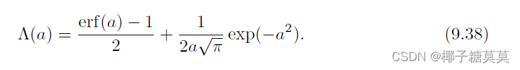
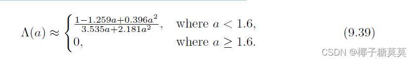
Equation 9.38 is expensive to evaluate since it includes erf, the error function. For this reason, an approximation [1833] is typically used instead: 

由于方程9.38包含了误差函数erf，所以它的计算成本很高。因此，通常使用近似值[1833]:

The next NDF we will discuss is the Blinn-Phong NDF. It was widely used in computer graphics in the past, though in recent times it has been largely superseded by other distributions. The Blinn-Phong NDF is still used in cases where computation is at a premium (e.g., on mobile hardware) because it is less expensive to compute than the other NDFs discussed in this section. 

我们要讨论的下一个NDF是Blinn-Phong NDF。它在过去被广泛用于计算机图形中，尽管最近它已经被其他发行版所取代。Blinn-Phong NDF仍然用于计算成本较高的情况(例如在移动硬件上)，因为它的计算成本低于本节讨论的其他NDF。

The Blinn-Phong NDF was derived by Blinn [159] as a modification of the (nonphysically based) Phong shading model [1414]:

Blinn-Phong NDF是由Blinn [159]作为(基于非物理的)Phong着色模型[1414]的修改而得出的:

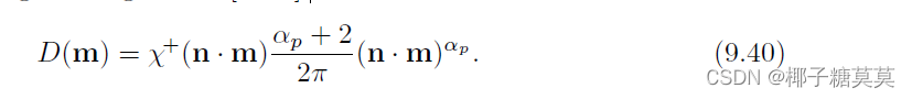
 The power αp is the roughness parameter of the Phong NDF. High values represent smooth surfaces and low values represent rough ones. The values of αp can go arbitrarily high for extremely smooth surfaces—a perfect mirror would require αp = ∞. A maximally random surface (uniform NDF) can be achieved by setting αp to 0. The αp parameter is not convenient to manipulate directly since its visual impact is highly nonuniform. Small numerical changes have large visual effects for small αp values, but large values can be changed significantly without much visual impact. For this reason, αp is typically derived from a user-manipulated parameter via a nonlinear mapping. For example, αp = pow(m, s), where s is a parameter value between 0 and 1 and m is an upper bound for αp in a given application. This mapping was used by several games, including Call of Duty: Black Ops, where m was set to a value of 8192 [998].

功率αp是Phong NDF的粗糙度参数。高值表示平滑的表面，低值表示粗糙的表面。对于极其光滑的表面，αp的值可以任意高——完美的镜面需要αp = ∞。通过将αp设置为0，可以获得最大的随机表面(均匀NDF)。αp参数不便于直接操作，因为它的视觉效果非常不均匀。对于较小的αp值，较小的数值变化具有较大的视觉效果，但是较大的值可以显著改变，而没有太大的视觉影响。为此，αp通常通过非线性映射从用户操作的参数中导出。例如，αp = pow(m, s),，其中s是0到1之间的参数值，m是给定应用中αp的上限。这种映射被几个游戏使用，包括使命召唤:黑色行动，其中m被设置为8192 [998]的值。

Such “interface mappings” are generally useful when the behavior of a BRDF parameter is not perceptually uniform. These mappings are used to interpret parameters set via sliders or painted in textures.

当BRDF参数的行为在感觉上不一致时，这种“接口映射”通常是有用的。这些映射用于解释通过滑块设置或绘制在纹理中的参数。

Equivalent values for the Beckmann and Blinn-Phong roughness parameters can be found using the relation [1833]. When the parameters are matched in this way, the two distributions are quite close, especially for relatively smooth surfaces, as can be seen in the upper left of Figure 9.36.

贝克曼和Blinn-Phong粗糙度参数的等效值可使用关系式[1833]找到。当参数以这种方式匹配时，两个分布非常接近，特别是对于相对光滑的表面，正如在图9.36的左上方可以看到的。

The Blinn-Phong NDF is not shape-invariant, and an analytic form does not exist for its  function. Walter et al. [1833] suggest using the Beckmann  function in conjunction with the parameter equivalence.

Blinn-Phong NDF不是形状不变的，并且其函数不存在解析形式。沃尔特等人[1833]建议将贝克曼函数与参数等效结合使用。

In the same 1977 paper [159] in which Blinn adapted the Phong shading function into a microfacet NDF, he proposed two other NDFs. Of these three distributions, Blinn recommended one derived by Trowbridge and Reitz [1788]. This recommendation was not widely heeded, but 30 years later the Trowbridge-Reitz distribution was independently rediscovered byWalter et al. [1833], who named it the GGX distribution. This time, the seed took root. Within a few years, adoption of the GGX distribution started spreading across the film [214, 1133] and game [861, 960] industries, and today it likely is the most often-used distribution in both. Blinn’s recommendation appears to have been 30 years ahead of its time. Although “Trowbridge-Reitz distribution” is technically the correct name, we use the GGX name in this book since it is firmly established.

在1977年的同一篇论文[159]中，Blinn将Phong着色函数应用到一个微曲面NDF中，他提出了另外两个NDF。在这三种分布中，Blinn推荐了一种由Trowbridge和Reitz [1788]导出的分布。这个建议没有被广泛注意，但是30年后，特罗布里奇-赖茨分布被沃尔特等人[1833]独立地重新发现，他将其命名为GGX分布。这一次，种子生根发芽了。几年内，GGX发行版的采用开始在电影[214，1133]和游戏[861，960]行业蔓延，今天它可能是这两个行业中最常用的发行版。Blinn的建议似乎超前了30年。虽然“特罗布里奇-赖茨分布”在技术上是正确的名称，我们在本书中使用GGX的名字，因为它是牢固建立的。

The GGX distribution is

GGX分布是

 

The roughness control provided by the αg parameter is similar to that provided by the Beckmann αb parameter. In the Disney principled shading model, Burley [214] exposes the roughness control to users as , where r is the user-interface roughness parameter value between 0 and 1. Exposing r as a slider value means that the effect changes in a more linear fashion. This mapping has been adopted by most applications that use the GGX distribution. 

αg参数提供的粗糙度控制类似于Beckmann αb参数提供的粗糙度控制。在迪士尼原则性阴影模型中，Burley [214]将粗糙度控制暴露给用户为，其中r是0到1之间的用户界面粗糙度参数值。将r显示为滑块值意味着效果以更线性的方式变化。大多数使用GGX分布的应用程序都采用了这种映射。

 The GGX distribution is shape-invariant, and its function is relatively simple:

 GGX分布是形状不变的，其函数相对简单:

 

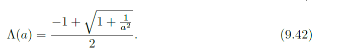
The fact that the variable a appears in Equation 9.42 only as pow(a, 2) is convenient, since the square root in Equation 9.37 can be avoided. 

 变量a在方程9.42中只作为pow(a，2)出现是方便的，因为方程9.37中的平方根可以避免。

 Due to the popularity of the GGX distribution and the Smith masking-shadowing function, there has been a focused effort to optimize the combination of the two. Lagarde observes [960] that the height-correlated Smith G2 for GGX (Equation 9.31) has terms that cancel out when combined with the denominator of the specular microfacet BRDF (Equation 9.34). The combined term can be simplified thusly:

由于GGX分布和史密斯掩蔽-遮蔽函数的流行，已经集中努力来优化这两者的组合。Lagarde观察到[960]GGX(方程9.31)的高度相关的Smith G2在与镜面微表面BRDF(方程9.34)的分母结合时有抵消项。合并后的术语可以这样简化:

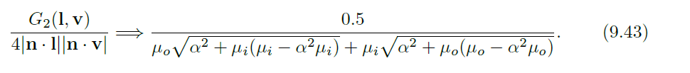
The equation uses the variable replacement μi = (n · l)+ and μo = (n · v)+ for brevity. Karis [861] proposes an approximated form of the Smith G1 function for GGX: 

为简便起见，该等式使用变量替换μi = (n · l)+和μo = (n · v)+来表示。Karis [861]提出了GGX的史密斯G1函数的近似形式:

where s can be replaced with either l or v. Hammon [657] shows that this approximated form of G1 leads to an efficient approximation for the combined term composed of the height-correlated Smith G2 function and the specular microfacet BRDF denominator: 

其中s可以用l或v代替。Hammon [657]表明，G1的这种近似形式可以有效地近似由高度相关的Smith G2函数和镜面微面BRDF分母组成的组合项:

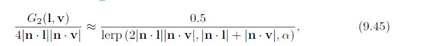
which uses the linear interpolation operator, lerp(x, y, s) = x(1 − s) + ys. 

它使用线性插值算子lerp(x, y, s) = x(1 − s) + ys。

When comparing the GGX and Beckmann distributions in Figure 9.36, it is apparent that the two have fundamentally different shapes. GGX has narrower peaks than Beckmann, as well as longer “tails” surrounding those peaks. In the rendered images at the bottom of the figure, we can see that GGX’s longer tails create the appearance of a haze or glow around the core of the highlight.

当比较图9.36中的GGX分布和贝克曼分布时，很明显，两者有根本不同的形状。GGX比贝克曼有更窄的峰，以及围绕这些峰的更长的“尾巴”。在图底部的渲染图像中，我们可以看到GGX较长的尾巴在高光的核心周围产生了薄雾或辉光的外观。

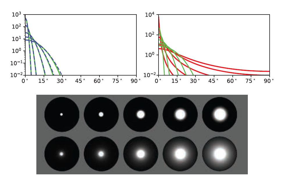
Figure 9.36. On the upper left, a comparison of Blinn-Phong (dashed blue) and Beckmann (green) distributions for values of αb ranging from 0.025 to 0.2 (using the parameter relation.On the upper right, a comparison of GGX (red) and Beckmann (green) distributions. The values of αb are the same as in the left plot. The values of αg have been adjusted by eye to match highlight size. These same values have been used in the spheres rendered on the bottom image. The top row uses the Beckmann NDF and the bottom row uses GGX. 

 图9.36。左上角是Blinn-Phong(蓝色虚线)和Beckmann(绿色)分布的比较，αb值范围为0.025至0.2(使用参数关系)。右上角是GGX(红色)和贝克曼(绿色)分布的比较。αb的值与左图中的值相同。αg的值已经由眼睛调整以匹配高光尺寸。这些相同的值已经被用于渲染在底部图像上的球体。顶行使用Beckmann NDF，底行使用GGX。 ​

Many real-world materials show similar hazy highlights, with tails that are typically longer even than those of the GGX distribution [214]. See Figure 9.37. This realization has been a strong contributor to the growing popularity of the GGX distribution, as well as the continuing search for new distributions that would fit measured materials even more accurately.

许多真实世界的材料显示了类似的模糊高光，其尾部通常比GGX分布的更长[214]。参见图9.37。这种认识极大地促进了GGX分布越来越受欢迎，以及对更精确地拟合测量材料的新分布的不断探索。

Figure 9.37. NDFs fit to measured chrome from the MERL database. On the left, we have plots of the specular peak against θm for chrome (black), GGX (red; αg = 0.006), Beckmann (green; αb = 0.013), and Blinn-Phong (blue dashes; n = 12000). Rendered highlights are shown on the right for chrome, GGX, and Beckmann. (Figure courtesy of Brent Burley [214].) 

图9.37。NDF适合MERL数据库中的测量铬。在左边，我们有铬(黑色)、GGX(红色；αg = 0.006)，贝克曼(绿色；αb = 0.013)，以及Blinn-Phong(蓝色破折号；n = 12000)。铬合金，GGX和贝克曼渲染的高光显示在右边。(图由布伦特·伯利提供[214]。)

Burley [214] proposed the generalized Trowbridge-Reitz (GTR) NDF with a goal of allowing for more control over the NDF’s shape, specifically the tails of the distribution:

Burley [214]提出了广义Trowbridge-Reitz (GTR) NDF，目的是对NDF的形状进行更多控制，特别是分布的尾部:

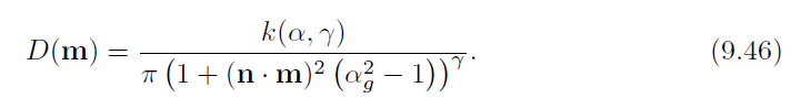
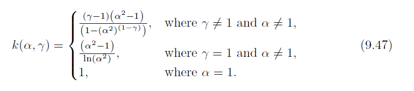
The γ argument controls the tail shape. When γ = 2, GTR is the same as GGX. As the value of γ decreases, tails of the distribution become longer, and as it increases, they become shorter. At high values of γ, the GTR distribution resembles Beckmann. The k(α, γ) term is the normalization factor, which we give in a separate equation, since it is more complicated than those of other NDFs: 

γ参数控制尾部形状。当γ = 2时，GTR与GGX相同。随着γ值的减小，分布的尾部变长，随着γ值的增大，尾部变短。在高γ值时，GTR分布类似贝克曼分布。k(α，γ)项是归一化因子，我们在单独的方程中给出，因为它比其他NDF更复杂:

The GTR distribution is not shape-invariant, which complicates finding its Smith G2 masking-shadowing function. It took three years after publication of the NDF for a solution for G2 to be published [355]. This G2 solution is quite complex, with a table of analytical solutions for certain values of γ (for intermediate values, interpolation must be used). Another issue with GTR is that the parameters α and γ affect the perceived roughness and “glow” in a non-intuitive manner. 

GTR分布不是形状不变的，这使得寻找它的Smith G2遮蔽函数变得复杂。NDF发布三年后，G2的解决方案才得以发布[355]。这个G2解相当复杂，有一个γ的某些值的解析解表(对于中间值，必须使用插值)。GTR的另一个问题是参数α和γ以非直观的方式影响感知的粗糙度和“辉光”。

Student’s t-distribution (STD) [1491] and exponential power distribution (EPD) [763] NDFs include shape control parameters. In contrast to GTR, these functions are shape-invariant with respect to their roughness parameters. At the time of writing, these are newly published, so it is not clear whether they will find use in applications.

学生的t分布(STD) [1491]和指数幂分布(EPD)[763]NDF包括形状控制参数。与GTR相反，这些函数相对于它们的粗糙度参数是形状不变的。在撰写本文时，这些都是新发表的，所以还不清楚它们是否会在应用中找到用途。

Instead of increasing the complexity of the NDF, an alternative solution to better matching measured materials is to use multiple specular lobes. This idea was suggested by Cook and Torrance [285, 286]. It was experimentally tested by Ngan [1271], who found that for many materials adding a second lobe did improve the fit significantly. Pixar’s PxrSurface material [732] has a “roughspecular” lobe that is intended to be used (in conjunction with the main specular lobe) for this purpose. The additional lobe is a full specular microfacet BRDF with all the associated parameters and terms. Imageworks employs a more surgical approach [947], using a mix of two GGX NDFs that are exposed to the user as an extended NDF, rather than an entire separate specular BRDF term. In this case, the only additional parameters needed are a second roughness value and a blend amount.

为了不增加NDF的复杂性，更好地匹配被测材料的另一种解决方案是使用多个镜面反射瓣。这个想法是由库克和托兰斯[285，286]提出的。Ngan [1271]对其进行了实验测试，他发现，对于许多材料来说，添加第二个波瓣确实显著提高了拟合度。Pixar的PxrSurface材质[732]有一个“粗糙镜面”波瓣，用于此目的(与主镜面波瓣结合使用)。附加波瓣是一个全镜面微表面BRDF，具有所有相关参数和术语。Imageworks采用了一种更加外科手术式的方法[947]，使用两种GGX NDF的混合，作为扩展的NDF暴露给用户，而不是整个单独的镜面BRDF项。在这种情况下，唯一需要的附加参数是第二个粗糙度值和混合量。

Anisotropic Normal Distribution Functions

各向异性正态分布函数

While most materials have isotropic surface statistics, some have significant anisotropy in their microstructure that noticeably affects their appearance, e.g., Figure 9.26 on page 329. To accurately render such materials, we need BRDFs, especially NDFs that are anisotropic as well.

虽然大多数材料具有各向同性的表面统计数据，但一些材料的微观结构具有显著的各向异性，这会显著影响其外观，例如，第329页的图9.26。为了精确渲染这些材质，我们需要BRDFs，尤其是各向异性的NDF。

Unlike isotropic NDFs, anisotropic NDFs cannot be evaluated with just the angle θm. Additional orientation information is needed. In the general case, the microfacet normal m needs to be transformed into the local frame or tangent space defined by the normal, tangent, and bitangent vectors, respectively, n, t, and b. See Figure 6.32 on page 210. In practice, this transformation is typically expressed as three separate dot products: m· n, m· t, and m· b.

与各向同性NDFs不同，各向异性NDFs不能仅通过角度θm进行评估，还需要额外的取向信息。在一般情况下，微法面法线m需要转换到局部坐标系或切线空间，分别由法线、切线和双切线向量n、t和b定义，见图6.32。实际上，这种转换通常表示为三个独立的点积:m· n, m· t, and m· b。

When combining normal mapping with anisotropic BRDFs, it is important to make sure that the normal map perturbs the tangent and bitangent vectors as well as the normal. This procedure is often done by applying the modified Gram-Schmidt process to the perturbed normal n and the interpolated vertex tangent and bitangent vectors t0 and b0 (the below assumes that n is already normalized):

当结合法线贴图和各向异性BRDFs时，确保法线贴图干扰切线和双切线向量以及法线是很重要的。这一过程通常通过将修改的Gram-Schmidt过程应用于扰动的法线n和插值的顶点切线和双切线向量t0和b0来完成(下面假设n已经被归一化):

Alternatively, after the first line the orthogonal b vector could be created by taking the cross product of n and t. 

或者，在第一行之后，正交b向量可以通过取n和t的交叉乘积来创建。 

For effects such as brushed metal or curly hair, per-pixel modification of the tangent direction is needed, typically provided by a tangent map. This map is a texture that stores the per-pixel tangent, similar to how a normal map stores per-pixel normals.Tangent maps most often store the two-dimensional projection of the tangent vector onto the plane perpendicular to the normal. This representation works well with texture filtering and can be compressed similar to normal maps. Some applications store a scalar rotation amount instead, which is used to rotate the tangent vector around n. Though this representation is more compact, it is prone to texture filtering artifacts where the rotation angle wraps around from 360◦ to 0◦.

对于金属拉丝或卷发等效果，需要对切线方向进行逐像素修改，通常由切线贴图提供。该贴图是一种存储每像素切线的纹理，类似于法线贴图存储每像素法线的方式。切线贴图通常将切线向量的二维投影存储在垂直于法线的平面上。这种表示法与纹理过滤配合得很好，并且可以像法线贴图一样压缩。一些应用存储标量旋转量，用于围绕n旋转切向量，虽然这种表示更紧凑，但在旋转角度从360°到0°的情况下，容易出现纹理过滤伪像。

A common approach to creating an anisotropic NDF is to generalize an existing isotropic NDF. The general approach used can be applied to any shape-invariant isotropic NDF [708], which is another reason why shape-invariant NDFs are preferable. Recall that isotropic shape-invariant NDFs can be written in the following form:

创建各向异性NDF的常见方法是推广现有的各向同性NDF。所用的一般方法可应用于任何形状不变的各向同性NDF [708]，这是形状不变NDF更可取的另一个原因。回想一下，各向同性的形状不变NDF可以写成以下形式:

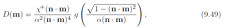
with g representing a one-dimensional function that expresses the shape of the NDF.The anisotropic version is 

其中g代表表示NDF形状的一维函数。 各向异性版本是

The parameters αx and αy represent the roughness along the direction of t and b, respectively. If αx = αy, Equation 9.50 reduces back to the isotropic form.

参数αx和αy分别表示沿t和b方向的粗糙度。如果αx = αy，方程9.50又回到各向同性形式。

The G2 masking-shadowing function for the anisotropic NDF is the same as the isotropic one, except that the variable a (passed into the function) is calculated differently:

各向异性NDF的G2掩蔽-遮蔽函数与各向同性的相同，只是变量a(传递到函数中)的计算方式不同:

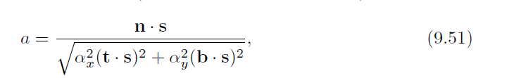
where (as in Equation 9.37) s represents either v or l.

其中(如方程式9.37) s代表v或l。

Using this method, anisotropic versions have been derived for the Beckmann NDF,

使用这种方法，已经为贝克曼NDF导出了各向异性版本，

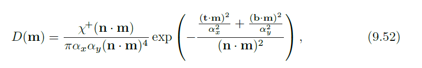
 and the GGX NDF,

和GGX NDF,

Both are shown in Figure 9.38. 

两者都如图9.38所示

 Figure 9.38. Spheres rendered with anisotropic NDFs: Beckmann in the top row and GGX in the bottom row. In both rows αy is held constant and αx is increased from left to right.

图9.38。使用各向异性NDF渲染的球体:贝克曼在顶行，GGX在底行。在两行中，αy保持不变，αx从左向右增加。

While the most straightforward way to parameterize anisotropic NDFs is to use the isotropic roughness parameterization twice, once for αx and once for αy, other parameterizations are sometimes used. In the Disney principled shading model [214], the isotropic roughness parameter r is combined with a second scalar parameter kaniso with a range of [0, 1]. The αx and αy values are computed from these parameters thusly:

虽然参数化各向异性NDF的最直接方法是使用两次各向同性粗糙度参数化，一次用于αx，一次用于αy，但有时也使用其他参数化。在迪士尼原则性阴影模型[214]中，各向同性粗糙度参数r与范围为[0，1]的第二标量参数kaniso组合。因此，αx和αy值由这些参数计算得出:

The 0.9 factor limits the aspect ratio to 10 : 1. 

0.9的系数将纵横比限制为10 : 1。

 Imageworks [947] use a different parameterization that allows for an arbitrary degree of anisotropy:

Imageworks [947]使用不同的参数化，允许任意程度的各向异性: