Anscombe's quartet

最新推荐文章于 2025-02-06 15:27:21 发布

Ouy_Kai

最新推荐文章于 2025-02-06 15:27:21 发布

阅读量661

点赞数

本文链接：https://blog.csdn.net/m0_37818428/article/details/80635448

版权

Python实践专栏收录该内容

13 篇文章

订阅专栏

本博客通过计算四个不同数据集的均值、方差及相关系数，并利用Seaborn进行可视化，展示了尽管统计数据相似，但数据分布却可能截然不同的现象。

摘要生成于 C知道，由 DeepSeek-R1 满血版支持，前往体验 >

题目描述

%matplotlib inline

import random

import numpy as np
import scipy as sp
import pandas as pd
import matplotlib.pyplot as plt
import seaborn as sns

import statsmodels.api as sm
import statsmodels.formula.api as smf

sns.set_context("talk")

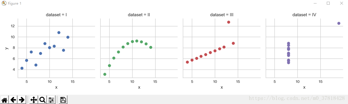
Anscombe’s quartet

Anscombe’s quartet comprises of four datasets, and is rather famous. Why? You’ll find out in this exercise.

anascombe = pd.read_csv('data/anscombe.csv')
anascombe.head()

dataset	x	y
0	10	8.04
1	8	6.95
2	13	7.58
3	9	8.81
4	11	8.33

Part 1

For each of the four datasets…

Compute the mean and variance of both x and y
Compute the correlation coefficient between x and y
Compute the linear regression line: y=β0+β1x+ϵ (hint: use statsmodels and look at the Statsmodels notebook)

Part 2

Using Seaborn, visualize all four datasets.

hint: use sns.FacetGrid combined with plt.scatter

解题代码

import numpy as np
import matplotlib.pyplot as plt
import seaborn as sns
import statsmodels.api as sm
import statistics as sta
import scipy.stats.stats as stats

anscombe = sns.load_dataset("anscombe")
print(anscombe)  # 打印原数据

str = ['I', 'II', 'III', 'IV']
Xarray = []
Yarray = []

for i in range(0, 4):
    array = anscombe.x[i * 11:i * 11 + 10].values   # 获取x的值，并打印
    Xarray.append(array)
    print("Xarray in " + str[i] + ":", Xarray[i])
    array = anscombe.y[i * 11:i * 11 + 10].values  # 获取x的值，并打印
    Yarray.append(array)
    print("Yarray in " + str[i] + ":", Yarray[i])

for i in range(0, 4):
    Xmean = np.mean(Xarray[i])   # 计算x的平均值，并打印
    print("mean of x in " + str[i] + ":", Xmean)
    Xvariance = sta.variance(Xarray[i])    # 计算x的方差，并打印
    print("variance of x in " + str[i] + ":", Xvariance)

print(' ')

for i in range(0, 4):
    Ymean = np.mean(Yarray[i])   # 计算y的平均值，并打印
    print("mean of x in " + str[i] + ":", Ymean)
    Yvariance = sta.variance(Yarray[i])    # 计算y的方差，并打印
    print("variance of x in " + str[i] + ":", Yvariance)

print('')

for i in range(0, 4):
    Cof = stats.pearsonr(Xarray[i], Yarray[i])[0]
    print("correlation coefficient of " + str[i] + ":", Cof)

print('')

for i in range(0, 4):
    X = sm.add_constant(Xarray[i])
    model = sm.OLS(Yarray[i], X)
    result = model.fit()
    params = result.params
    print("Dataset" + str[i] + ": y =", params[0], "+", params[1], "* x")

sns.set(style = 'whitegrid')  # 数据可视化，散点图
g = sns.FacetGrid(anscombe, col = "dataset", hue = "dataset", size = 3)
g.map(plt.scatter, 'x', 'y')
plt.show()

可视化结果

这里写图片描述