matlab绘制经典气体、玻色气体和费米气体的化学势随温度的变化曲线

前言

经典气体、玻色气体和费米气体的化学势随温度的变化曲线是热力学与统计物理中老生常谈的话题了，具有典型的代表性和对比性，下面简要介绍如何使用matlab绘制相关曲线，以及其算法演示。对于使用不同的画图软件和程序基本算法思路不变，但是一些程序命令需要读者根据软件的情况自行修改！

运行执行文件：

clc,clear;

% Classical particle
k = 1.380649*10^(-23);
h = 1.05457266*10^(-34);
syms T
u_classcial = T*log(T^(-3/2)*(2*pi)^(3/2));
fplot(u_classcial,[0,22],'r','LineWidth',1);hold on;

% Fermion
syms e2 u2
%ft = (e2.^(1/2))./(exp((e2-u2)./T)+1);
%N2 = integral(@(e2)ft,0,inf);
%fz = @(u2)N2-13.96;
t = 0.1:0.1:22;
i = 1;
u_fermi = [];
for T = 0.1:0.1:22
    u_fermi(i) = fzero(@(u2)integral(@(e2) (e2.^(1/2))./(exp((e2-u2)./T)+1),0,inf)-13.96,1);
    i = i+1;
end
plot(t,u_fermi,'b','LineWidth',1);hold on;

% Boson
fz0=g(3/2,1);
Tc=fz0^(-2/3)*2*pi;
z=0.15:0.05:1;
t=[];
for i=1:length(z)
t(i)=g(3/2,z(i));
end
t=t.^(-2/3)*2*pi;
u_bose = log(z).*t;

% Plot
plot(t,u_bose,'c','LineWidth',1);hold on;
plot(linspace(0,Tc,10),linspace(0,0,10),'c','LineWidth',1)
%line([Tc,Tc], [7,-41],'LineStyle','--','color', 'g','LineWidth',0.7);hold on;
%line([4,22], [0,0],'LineStyle','-.', 'color', 'm','LineWidth',0.1);
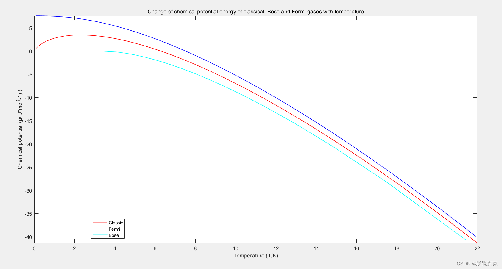
title('Change of chemical potential energy of classical, Bose and Fermi gases with temperature');
legend('Classic','Fermi','Bose','Location','best')
xlabel('Temperature (T/K)');
ylabel('Chemical potential (μ/ J*mol^(-1) )');

调用到的function文件：（玻色爱因斯坦函数）

function g=g(v,z)
syms x
g=double(symsum(z^x/x^v,x,1,inf));
end

绘制完成后的图像演示：

感谢阅读，有帮助点赞收藏支持呀~
有问题可以私信~