


此博客仅是学习笔记和个人学习心得总结
1、matlab代码——交互式画图示例
clear all
clc
f=input('frequency in Hz >>')
A=input('amplitude(>0) >>')
theta=input('phase in degrees >>')
omega= 2*pi*f;                                    %频率 rad/s
tmax = 1/f;                                       %一个周期
time=[];n=0;                                      %初始化
figure(1)
for t=0:tmax/36:tmax
    z=A*exp(1i*(omega*t+theta*pi/180));
    x=real(z);y=imag(z);
    time=[time t];
    subplot(121)
    compass(x,y);
    axis('square')
    subplot(122)
    plot(n*tmax/36,x,'*r')
    axis('square');
    axis([0 tmax -1.1*A 1.1*A]);grid
    hold on
    if n==0
        pause(1)
    else
        pause(0.1)
    end
        n=n+1;
end
hold off
2、处理二维信号——火车信号
%加载测试序列
%%
clear all;
clc
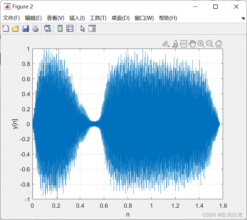
load train
whos
sound(y,Fs) %聆听并绘制火车信号
t=0:1/Fs:(length(y)-1)/Fs;
figure(2);plot(t,y');grid
ylabel('y[n]');xlabel('n')
%用函数绘制火车信号的200个样本
%%
figure(3)
n=100:299;
stem(n,y(100:299)):xlabel('n'):ylabel('y[n]')
title('火车信号片段')
axis([100 299 -0.5 0.5])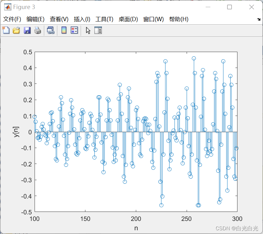
3、显示灰度图像
clear all
load clown
colormap('gray')
image(X)   %X实质就是关于图像的数字矩阵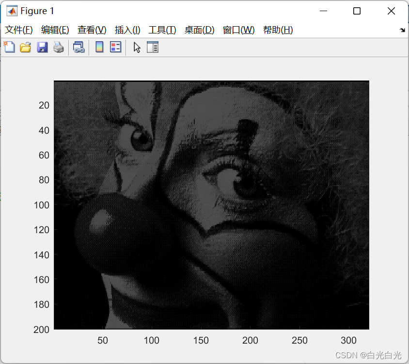
%重零开始创建一个WAV文件并回放
%%
clear all

Fs= 5000;                                         %抽样频率
t=0:1/Fs:5;                                       %时间参数
y=0.1*cos(2*pi*2000*t)-0.8*cos(2*pi*2000*t.^2);   %正弦和线性调频参数
%%写入chrip.wav文件
audiowrite('chrip.wav',y,Fs)
%%
[y1,Fs]=audioread('chrip.wav');
%注意老版本使用的是wavwrite和wavread,格式与audiowrite,autoread略微不同
sound(y1,Fs)                                      %产生声音
figure(4)
plot(t(1:1000),y1(1:1000))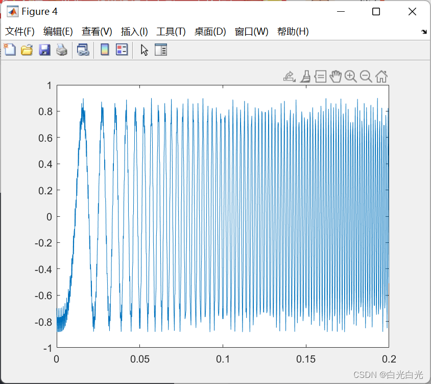
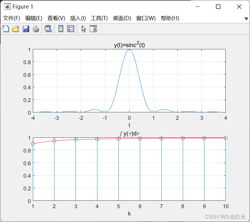
4、sinc函数
sinc函数在信号与系统理论中占有非常重要的地位,它的定义如下:
y(t)=sin(pi)t/(pi)t, 负无穷<t<正无穷
%平方sinc函数的积分
%%
clf;clear all
%符号型
syms t  z
for k=1:10
    z=int(sinc(t)^2,t,0,k);        %sinc^2的积分,从0到k
    zz(k)=subs(2*z);               %转换成数值型zz
end
%数值型
t1=linspace(-4,4);                 %区间[-4,4]内均匀分布100个点
y=sinc(t1).^2;                     %平方sinc函数的数值型定义
n=1:10
figure(1)
subplot(211)
plot(t1,y);
grid;
title('y(t)=sinc^2(t)');
xlabel('t')
subplot(212)
stem(n(1:10),zz(1:10));hold on
plot(n(1:10),zz(1:10),'r');grid;title('\int y(\tau)d\tau');hold off
xlabel('k')
图示显示sinc(t)^2的积分很快达到了1
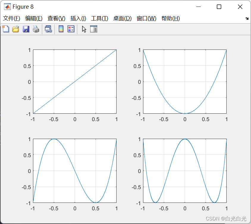
5、切比雪夫多项式和李萨如图形
%切比雪夫多项式
%%
clf
syms x y t
x= cos(2*pi*t);
figure(8)
for k=1:4
    y=cos(2*pi*k*t);
    if k==1,subplot(221)
        elseif k==2, subplot(222)
        elseif k==3, subplot(223)
            else subplot(224);
    end
    fplot(x,y);                %不推荐使用ezplot,图示对应于n=1,2,3,4的情形
    grid;
    hold on
end
hold off
%李萨如图形
%%
clear all;clf
syms x y t
x=cos(2*pi*t);
A=1;figure(9)
for i = 1:2
    for k=0:3
        theta=k*pi/4;
        y=A^k*cos(2*pi*t+theta);
        if k==0,subplot(221)
            elseif k==1,subplot(222)
            elseif k==2,subplot(223)
            else subplot(224);
        end
        fplot(x,y);
        grid;
        hold on
    end
        A=0.5;figure(10)
end
图示对应于n=1,2,3,4的切比雪夫多项式的情形
情况1(上半部由左向右)具有相同的振幅和输入和输出(A=1),但是相位差分别是0,pi/4,pi/2,3pi/4,情况2(下部分4个图由左向右)输入具有相同单位振幅,但是输出的振幅逐渐减少,相位差与情况一相同。
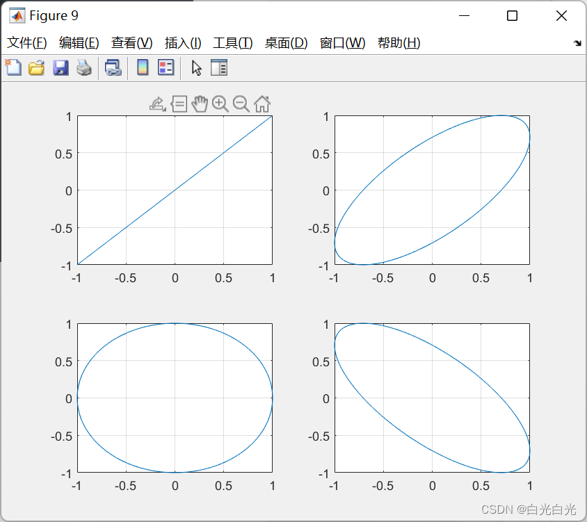
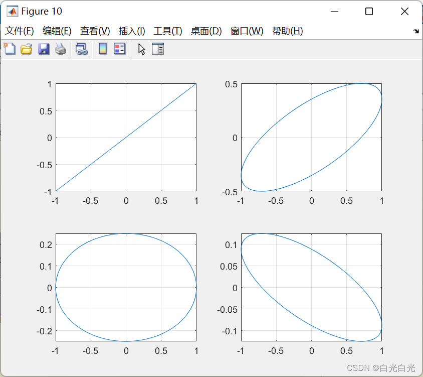
(注意坐标值的不同)
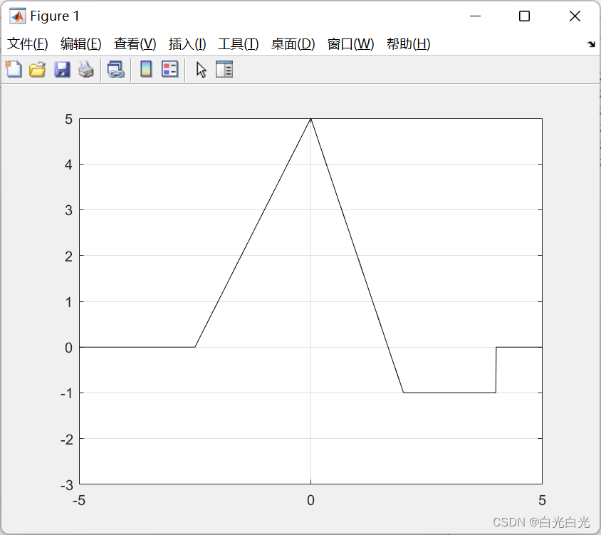
6,信号产生
%函数功能:用来产生一个斜变函数,输入为时间t,斜率m和平移量ad
%如果ad为正数,则表示往左平移
%这里的t也需要注意,是有意义的,他表示支持区间。

%单位斜坡信号
function y=ramp(t,m,ad)
N=length(t);
y=zeros(1,N);
for i=1:N
    if t(i)>=-ad
        y(i)=m*(t(i)+ad);
    end
end
end


%单位冲激函数
function y=ustep(t,ad)
N=length(t);
y=zeros(1,N);
for i=1:N
    if t(i)>=-ad
        y(i)=1;
    end
end
end
%偶/奇分解
%%
[ye,yo] = evenodd(t,y);
subplot(211)
plot(t,ye,'r')
grid

subplot(212)
plot(t,yo,'r')
grid
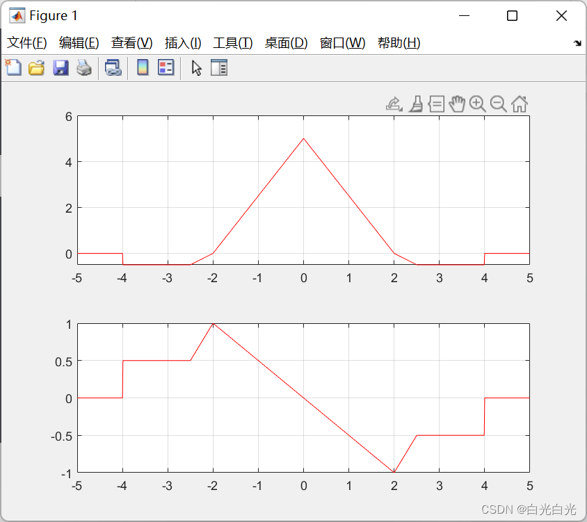
将原始信号分解出一个奇信号和一个偶信号,matlab函数fliplr将向量y的值反转过来产生反褶信号。
%(a)产生y(t)及其包络线
%%
t = sym('t');
y = exp(-t)*cos(2*pi*t);
ye = exp(-t);
figure(1)
fplot(y,2:4);
grid
hold on
fplot(ye,[-2,4])
hold on
fplot(-ye,[-2,4]);axis([-2 4 -8 8])
hold off
xlabel('t');ylabel('y(t)');title('')
% (b)产生x(t)
figure(2)
t = sym('t');
x = 1+1.5*cos(2*pi*t/10)-.6*cos(4*pi*t/10);
fplot(x,[-10,10]);grid
xlabel('t');ylabel('x(t)')
7,用matlab求卷积
clear all;
Ts=0.01;delay=1;Tend=2.5;t=0:Ts:Tend;
%(a)
x1=ustep(t,0)-ustep(t,-delay);h1=ustep(t,0)-ustep(t,-2*delay);
%(b)
x2=ramp(t,1,0)+ramp(t,-2,-1)+ramp(t,1,-2);h2=x2;
%(c)
x3=exp(-1*t);h3=exp(-10*t);
y=Ts*conv(x3,h3);                            %对于另外两种情况,修改x1和h1
t1=0:Ts:length(y)*Ts-Ts;
figure (1)
subplot(311)
plot(t,x3);axis([0 2.5 -0.1 1.2]);grid;ylabel('x_1(t)');
subplot(312)
plot(t,h3);axis([0 2.5 -0.1 1.2]);grid;ylabel('h_1(t)');
subplot(313)
plot(t1,y);
axis([0   5  -0.1 1.1]);
grid;
ylabel('y_1(t)');
x1 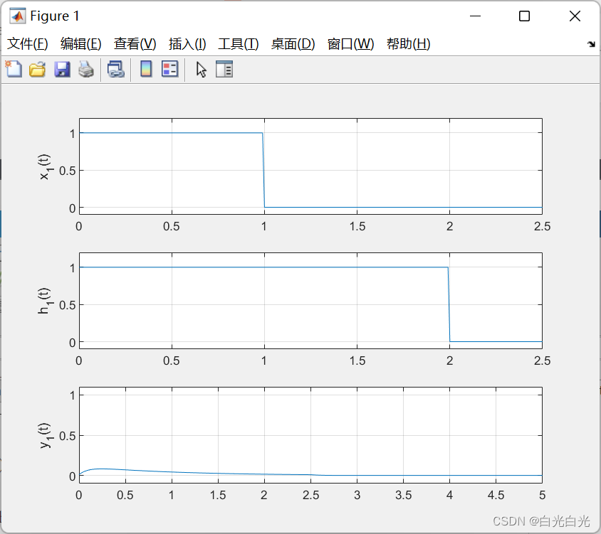 x2
x2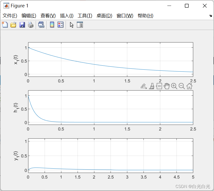
x3 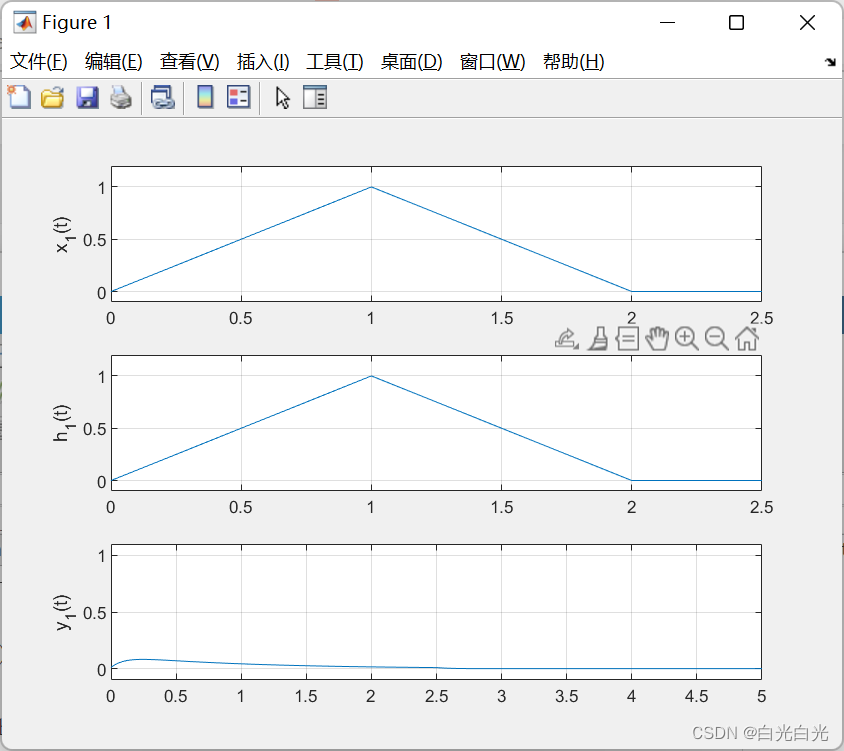


 1891
1891


 被折叠的 条评论
为什么被折叠?
被折叠的 条评论
为什么被折叠?
 到【灌水乐园】发言


