


先自我介绍一下,小编浙江大学毕业,去过华为、字节跳动等大厂,目前阿里P7
深知大多数程序员,想要提升技能,往往是自己摸索成长,但自己不成体系的自学效果低效又漫长,而且极易碰到天花板技术停滞不前!
因此收集整理了一份《2024年最新Python全套学习资料》,初衷也很简单,就是希望能够帮助到想自学提升又不知道该从何学起的朋友。


既有适合小白学习的零基础资料,也有适合3年以上经验的小伙伴深入学习提升的进阶课程,涵盖了95%以上Python知识点,真正体系化!
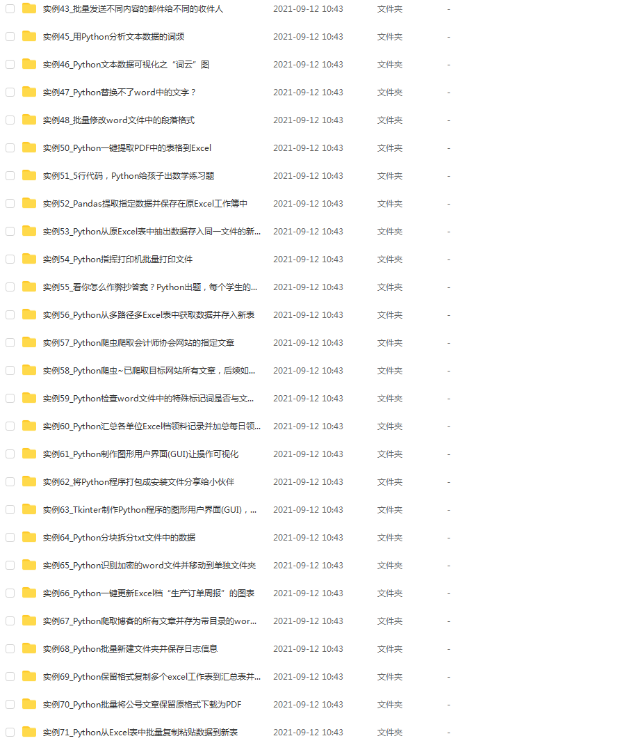
由于文件比较多,这里只是将部分目录截图出来,全套包含大厂面经、学习笔记、源码讲义、实战项目、大纲路线、讲解视频,并且后续会持续更新
如果你需要这些资料,可以添加V获取:vip1024c (备注Python)

正文
print(‘Coefficients:’, lin_reg_2.coef_) #查看回归方程系数(k)
print(‘intercept:’, lin_reg_2.intercept_) ##查看回归方程截距(b)
print(‘the model is y={0}+({1}*x)+({2}*x^2)’.format(lin_reg_2.intercept_,lin_reg_2.coef_[0],lin_reg_2.coef_[1]))
图像中显示
plt.scatter(datasets_X, datasets_Y, color = ‘red’) #scatter函数用于绘制数据点,这里表示用红色绘制数据点;
#plot函数用来绘制回归线,同样这里需要先将X处理成多项式特征;
plt.plot(X, lin_reg_2.predict(poly_reg.fit_transform(X)), color = ‘blue’)
plt.xlabel(‘Area’)
plt.ylabel(‘Price’)
plt.show()
3.3 结果
[[1.0000000e+00 1.0000000e+03 1.0000000e+06]
[1.0000000e+00 7.9200000e+02 6.2726400e+05]
[1.0000000e+00 1.2600000e+03 1.5876000e+06]
[1.0000000e+00 1.2620000e+03 1.5926440e+06]
[1.0000000e+00 1.2400000e+03 1.5376000e+06]
[1.0000000e+00 1.1700000e+03 1.3689000e+06]
[1.0000000e+00 1.2300000e+03 1.5129000e+06]
[1.0000000e+00 1.2550000e+03 1.5750250e+06]
[1.0000000e+00 1.1940000e+03 1.4256360e+06]
[1.0000000e+00 1.4500000e+03 2.1025000e+06]
[1.0000000e+00 1.4810000e+03 2.1933610e+06]
[1.0000000e+00 1.4750000e+03 2.1756250e+06]
[1.0000000e+00 1.4820000e+03 2.1963240e+06]
[1.0000000e+00 1.4840000e+03 2.2022560e+06]
[1.0000000e+00 1.5120000e+03 2.2861440e+06]
[1.0000000e+00 1.6800000e+03 2.8224000e+06]
[1.0000000e+00 1.6200000e+03 2.6244000e+06]
[1.0000000e+00 1.7200000e+03 2.9584000e+06]
[1.0000000e+00 1.8000000e+03 3.2400000e+06]
[1.0000000e+00 4.4000000e+03 1.9360000e+07]
[1.0000000e+00 4.2120000e+03 1.7740944e+07]
[1.0000000e+00 3.9200000e+03 1.5366400e+07]
[1.0000000e+00 3.2120000e+03 1.0316944e+07]
[1.0000000e+00 3.1510000e+03 9.9288010e+06]
[1.0000000e+00 3.1000000e+03 9.6100000e+06]
[1.0000000e+00 2.7000000e+03 7.2900000e+06]
[1.0000000e+00 2.6120000e+03 6.8225440e+06]
[1.0000000e+00 2.7050000e+03 7.3170250e+06]
[1.0000000e+00 2.5700000e+03 6.6049000e+06]
[1.0000000e+00 2.4420000e+03 5.9633640e+06]
[1.0000000e+00 2.3870000e+03 5.6977690e+06]
[1.0000000e+00 2.2920000e+03 5.2532640e+06]
[1.0000000e+00 2.3080000e+03 5.3268640e+06]
[1.0000000e+00 2.2520000e+03 5.0715040e+06]
[1.0000000e+00 2.2020000e+03 4.8488040e+06]
[1.0000000e+00 2.1570000e+03 4.6526490e+06]
[1.0000000e+00 2.1400000e+03 4.5796000e+06]
[1.0000000e+00 4.0000000e+03 1.6000000e+07]
[1.0000000e+00 4.2000000e+03 1.7640000e+07]
[1.0000000e+00 3.9000000e+03 1.5210000e+07]
[1.0000000e+00 3.5440000e+03 1.2559936e+07]
[1.0000000e+00 2.9800000e+03 8.8804000e+06]
[1.0000000e+00 4.3550000e+03 1.8966025e+07]
[1.0000000e+00 3.1500000e+03 9.9225000e+06]
[1.0000000e+00 3.0250000e+03 9.1506250e+06]
[1.0000000e+00 3.4500000e+03 1.1902500e+07]
[1.0000000e+00 4.4020000e+03 1.9377604e+07]
[1.0000000e+00 3.4540000e+03 1.1930116e+07]
[1.0000000e+00 8.9000000e+02 7.9210000e+05]]
[231.16788093 231.19868474 231.22954958 … 739.2018995 739.45285011
739.70386176]
Coefficients: [ 0.00000000e+00 -1.75650177e-02 3.05166076e-05]
intercept: 225.93740561055927
the model is y=225.93740561055927+(0.0x)+(-0.017565017675036532x^2)
3.4 可视化

4 案例实现——方法2
4.1 代码
numpy中np.array()与np.asarray的区别以及.tolist与np.asarray的区别以及.tolist")
import matplotlib.pyplot as plt
from sklearn.preprocessing import PolynomialFeatures
from sklearn.pipeline import Pipeline
from sklearn.linear_model import LinearRegression
from sklearn.metrics import mean_squared_error, r2_score
import numpy as np
import pandas as pd
import warnings
warnings.filterwarnings(action=“ignore”, module=“sklearn”)
dataset = pd.read_csv(‘多项式线性回归.csv’)
X = np.asarray(dataset.get(‘x’))
y = np.asarray(dataset.get(‘y’))
划分训练集和测试集
X_train = X[:-2]
X_test = X[-2:]
y_train = y[:-2]
y_test = y[-2:]
fit_intercept 为 True
model1 = Pipeline([(‘poly’, PolynomialFeatures(degree=2)), (‘linear’, LinearRegression(fit_intercept=True))])
model1 = model1.fit(X_train[:, np.newaxis], y_train)
y_test_pred1 = model1.named_steps[‘linear’].intercept_ + model1.named_steps[‘linear’].coef_[1] * X_test
print(‘while fit_intercept is True:…’)
print('Coefficients: ', model1.named_steps[‘linear’].coef_)
print(‘Intercept:’, model1.named_steps[‘linear’].intercept_)
print('the model is: y = ', model1.named_steps[‘linear’].intercept_, ’ + ', model1.named_steps[‘linear’].coef_[1],
‘* X’)
均方误差
print(“Mean squared error: %.2f” % mean_squared_error(y_test, y_test_pred1))
r2 score,0,1之间,越接近1说明模型越好,越接近0说明模型越差
print(‘Variance score: %.2f’ % r2_score(y_test, y_test_pred1), ‘\n’)
fit_intercept 为 False
model2 = Pipeline([(‘poly’, PolynomialFeatures(degree=2)), (‘linear’, LinearRegression(fit_intercept=False))])
model2 = model2.fit(X_train[:, np.newaxis], y_train)
y_test_pred2 = model2.named_steps[‘linear’].coef_[0] + model2.named_steps[‘linear’].coef_[1] * X_test + \
model2.named_steps[‘linear’].coef_[2] * X_test * X_test
print(‘while fit_intercept is False:…’)
print('Coefficients: ', model2.named_steps[‘linear’].coef_)
print(‘Intercept:’, model2.named_steps[‘linear’].intercept_)
print('the model is: y = ', model2.named_steps[‘linear’].coef_[0], ‘+’, model2.named_steps[‘linear’].coef_[1], '* X + ',
model2.named_steps[‘linear’].coef_[2], ‘* X^2’)
均方误差
print(“Mean squared error: %.2f” % mean_squared_error(y_test, y_test_pred2))
r2 score,0,1之间,越接近1说明模型越好,越接近0说明模型越差
print(‘Variance score: %.2f’ % r2_score(y_test, y_test_pred2), ‘\n’)
plt.xlabel(‘x’)
plt.ylabel(‘y’)
画训练集的散点图
plt.scatter(X_train, y_train, alpha=0.8, color=‘black’)
画模型
plt.plot(X_train, model2.named_steps[‘linear’].coef_[0] + model2.named_steps[‘linear’].coef_[1] * X_train +
model2.named_steps[‘linear’].coef_[2] * X_train * X_train, color=‘red’,
linewidth=1)
plt.show()
4.2 结果
如果不用框架,需要自己手动对数据添加高阶项,有了框架就方便多了。sklearn 使用 Pipeline 函数简化这部分预处理过程。
当 PolynomialFeatures 中的degree=1时,效果和使用 LinearRegression 相同,得到的是一个线性模型,degree=2时,是二次方程,如果是单变量的就是抛物线,双变量的就是抛物面。以此类推。
这里有一个 fit_intercept 参数,下面通过一个例子看一下它的作用。
当 fit_intercept 为 True 时,coef_ 中的第一个值为 0,intercept_ 中的值为实际的截距。
当 fit_intercept 为 False 时,coef_ 中的第一个值为截距,intercept_ 中的值为 0。
如图,第一部分是 fit_intercept 为 True 时的结果,第二部分是 fit_intercept 为 False 时的结果。
while fit_intercept is True:…
Coefficients: [ 0.00000000e+00 -3.70858180e-04 2.78609637e-05]
Intercept: 204.25470490804574
the model is: y = 204.25470490804574 + -0.00037085818009180454 * X
Mean squared error: 26964.95
Variance score: -3.61
while fit_intercept is False:…
Coefficients: [ 2.04254705e+02 -3.70858180e-04 2.78609637e-05]
Intercept: 0.0
the model is: y = 204.2547049080572 + -0.0003708581801012066 * X + 2.7860963722809286e-05 * X^2
Mean squared error: 7147.78
Variance score: -0.22
4.3 可视化
文末有福利领取哦~
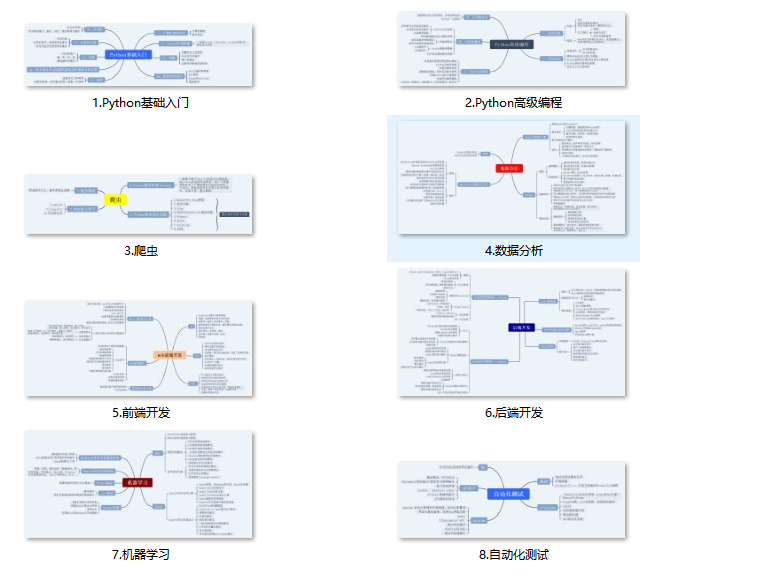
👉一、Python所有方向的学习路线
Python所有方向的技术点做的整理,形成各个领域的知识点汇总,它的用处就在于,你可以按照上面的知识点去找对应的学习资源,保证自己学得较为全面。
👉二、Python必备开发工具

👉三、Python视频合集
观看零基础学习视频,看视频学习是最快捷也是最有效果的方式,跟着视频中老师的思路,从基础到深入,还是很容易入门的。

👉 四、实战案例
光学理论是没用的,要学会跟着一起敲,要动手实操,才能将自己的所学运用到实际当中去,这时候可以搞点实战案例来学习。(文末领读者福利)

👉五、Python练习题
检查学习结果。

👉六、面试资料
我们学习Python必然是为了找到高薪的工作,下面这些面试题是来自阿里、腾讯、字节等一线互联网大厂最新的面试资料,并且有阿里大佬给出了权威的解答,刷完这一套面试资料相信大家都能找到满意的工作。


👉因篇幅有限,仅展示部分资料,这份完整版的Python全套学习资料已经上传
网上学习资料一大堆,但如果学到的知识不成体系,遇到问题时只是浅尝辄止,不再深入研究,那么很难做到真正的技术提升。
需要这份系统化的资料的朋友,可以添加V获取:vip1024c (备注python)

一个人可以走的很快,但一群人才能走的更远!不论你是正从事IT行业的老鸟或是对IT行业感兴趣的新人,都欢迎加入我们的的圈子(技术交流、学习资源、职场吐槽、大厂内推、面试辅导),让我们一起学习成长!
mg.cn/a9d7c35e6919437a988883d84dcc5e58.png)
👉因篇幅有限,仅展示部分资料,这份完整版的Python全套学习资料已经上传
网上学习资料一大堆,但如果学到的知识不成体系,遇到问题时只是浅尝辄止,不再深入研究,那么很难做到真正的技术提升。
需要这份系统化的资料的朋友,可以添加V获取:vip1024c (备注python)
[外链图片转存中…(img-tiZpv08D-1713450095521)]
一个人可以走的很快,但一群人才能走的更远!不论你是正从事IT行业的老鸟或是对IT行业感兴趣的新人,都欢迎加入我们的的圈子(技术交流、学习资源、职场吐槽、大厂内推、面试辅导),让我们一起学习成长!


 1046
1046

 被折叠的 条评论
为什么被折叠?
被折叠的 条评论
为什么被折叠?
 到【灌水乐园】发言


