CycleGAN详解与实现（采用tensorflow2

感谢每一个认真阅读我文章的人，看着粉丝一路的上涨和关注，礼尚往来总是要有的：

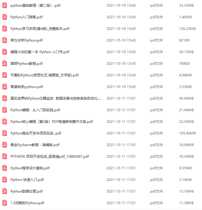
①　2000多本Python电子书（主流和经典的书籍应该都有了）

②　Python标准库资料（最全中文版）

③　项目源码（四五十个有趣且经典的练手项目及源码）

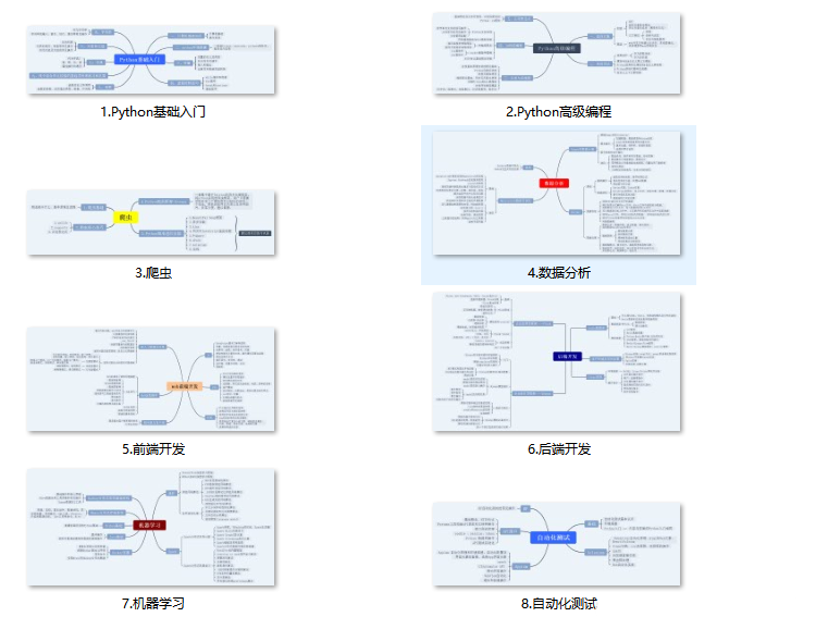
④　Python基础入门、爬虫、web开发、大数据分析方面的视频（适合小白学习）

⑤ Python学习路线图（告别不入流的学习）

网上学习资料一大堆，但如果学到的知识不成体系，遇到问题时只是浅尝辄止，不再深入研究，那么很难做到真正的技术提升。

需要这份系统化学习资料的朋友，可以戳这里获取

一个人可以走的很快，但一群人才能走的更远！不论你是正从事IT行业的老鸟或是对IT行业感兴趣的新人，都欢迎加入我们的的圈子（技术交流、学习资源、职场吐槽、大厂内推、面试辅导），让我们一起学习成长！

前向循环CycleGAN的目的是学习：

y ′ = G ( x ) ( 1 ) y’=G(x) \qquad(1) y′=G(x)(1)

要训练生成器，必须构建一个GAN。 这就是前向循环GAN，像典型GAN一样，由生成器 G G G和鉴别器 D y D_y Dy​组成，可以以相同的对抗方式对其进行训练。 通过仅利用源域中的图像 x x x和目标域中的图像 y y y来进行无监督学习。

与常规GAN不同，CycleGAN施加了循环一致性约束，前向循环一致性网络确保可以从伪造的目标数据中重建真实的源数据：

这是通过最小化前向循环一致性 L 1 L_1 L1​损失来完成的：

L f o r w a r d − c y c = E x ∼ p d a t a ( x ) [ ∥ F ( G ( x ) ) − x ∥ 1 ] ( 2 ) \mathcal L_{forward-cyc}= \mathbb E_{x\sim p_{data}(x)}[\| F(G(x))-x\|_1] \qquad (2) Lforward−cyc​=Ex∼pdata​(x)​[∥F(G(x))−x∥1​](2)

循环一致性损失使用 L 1 L_1 L1​或平均绝对误差（MAE），因为与 L 2 L_2 L2​或均方误差（MSE）相比，它通常导致较少的图像重建模糊。

循环一致性检查表明，尽管已将源数据 x x x转换为域 y y y，但 x x x的原始特征应在 y y y中保持不变并可以恢复。 网络F是从反向循环GAN借用的另一个生成器。

反向循环

CycleGAN是对称的。反向循环GAN与前向循环GAN相同，但是源数据 x x x和目标数据 y y y相反。 源数据为 y y y，目标数据为 x x x。生成器 G G G和 F F F的作用也相反。 F F F变为是生成器，而 G G G用于恢复输入。在前向循环GAN中，生成器 F F F是用于恢复源数据的网络，而 G G G是生成器。

反向循环GAN生成器的目标是合成：

x ′ = F ( y ) ( 3 ) x’=F(y)\qquad(3) x′=F(y)(3)

这可以通过对抗性训练反向循环GAN来完成。 目的是使生成器 F F F学习如何欺骗鉴别器 D x D_x Dx​。

此外，还具有类似的反向循环一致性以恢复原始源 y y y：

y ′ = G ( F ( y ) ) ( 4 ) y’=G(F(y))\qquad(4) y′=G(F(y))(4)

这是通过最小化反向循环一致性 L 1 L_1 L1​损失来完成的：

L b a c k w a r d − c y c = E y ∼ p d a t a ( y ) [ ∥ G ( F ( y ) ) − y ∥ 1 ] ( 5 ) \mathcal L_{backward-cyc}= \mathbb E_{y\sim p_{data}(y)}[\| G(F(y))-y\|_1] \qquad (5) Lbackward−cyc​=Ey∼pdata​(y)​[∥G(F(y))−y∥1​](5)

CycleGAN的最终目标是让生成器 G G G学习如何合成伪造的目标数据 y ′ y’ y′，该伪造的目标数据 y ′ y’ y′使用前向循环的鉴别器 D y D_y Dy​。 由于网络是对称的，因此CycleGAN还希望生成器 F F F学习如何合成伪造的源数据 x ′ x’ x′，该伪造的源数据 x ′ x’ x′可以在反向循环中欺骗鉴别器 D x D_x Dx​。

受最小二乘GAN（LSGAN）更好的感知质量的启发，CycleGAN的鉴别器和生成器还使用MSE损失。 LSGAN与原始GAN之间的差异是使用MSE损失，而不是二元交叉熵损失。

训练过程

CycleGAN将生成器－鉴别器损失函数表示为：

L f o r w a r d − G A N ( D ) = E y ∼ p d a t a ( y ) ( D y ( y ) − 1 ) 2 + E x ∼ p d a t a ( x ) D y ( G ( x ) ) 2 ( 6 ) \mathcal L_{forward-GAN}^{(D)}= \mathbb E_{y\sim p_{data}(y)}(D_y(y)-1)^2+ \mathbb E_{x\sim p_{data}(x)}D_y(G(x))^2\qquad (6) Lforward−GAN(D)​=Ey∼pdata​(y)​(Dy​(y)−1)2+Ex∼pdata​(x)​Dy​(G(x))2(6)

L f o r w a r d − G A N ( G ) = E x ∼ p d a t a ( x ) ( D y ( G ( x ) ) − 1 ) 2 ( 7 ) \mathcal L_{forward-GAN}^{(G)}= \mathbb E_{x\sim p_{data}(x)}(D_y(G(x))-1)^2\qquad (7) Lforward−GAN(G)​=Ex∼pdata​(x)​(Dy​(G(x))−1)2(7)

L b a c k w a r d − G A N ( D ) = E x ∼ p d a t a ( x ) ( D x ( x ) − 1 ) 2 + E y ∼ p d a t a ( y ) D x ( G ( y ) ) 2 ( 8 ) \mathcal L_{backward-GAN}^{(D)}= \mathbb E_{x\sim p_{data}(x)}(D_x(x)-1)^2+ \mathbb E_{y\sim p_{data}(y)}D_x(G(y))^2\qquad (8) Lbackward−GAN(D)​=Ex∼pdata​(x)​(Dx​(x)−1)2+Ey∼pdata​(y)​Dx​(G(y))2(8)

L b a c k w a r d − G A N ( G ) = E y ∼ p d a t a ( y ) ( D x ( G ( y ) ) − 1 ) 2 ( 9 ) \mathcal L_{backward-GAN}^{(G)}= \mathbb E_{y\sim p_{data}(y)}(D_x(G(y))-1)^2\qquad (9) Lbackward−GAN(G)​=Ey∼pdata​(y)​(Dx​(G(y))−1)2(9)

L G A N ( D ) = L f o r w a r d − G A N ( D ) + L b a c k w a r d − G A N ( D ) ( 10 ) \mathcal L_{GAN}^{(D)}=\mathcal L_{forward-GAN}^{(D)}+\mathcal L_{backward-GAN}^{(D)}\qquad(10) LGAN(D)​=Lforward−GAN(D)​+Lbackward−GAN(D)​(10)

L G A N ( G ) = L f o r w a r d − G A N ( G ) + L b a c k w a r d − G A N ( G ) ( 11 ) \mathcal L_{GAN}^{(G)}=\mathcal L_{forward-GAN}^{(G)}+\mathcal L_{backward-GAN}^{(G)}\qquad(11) LGAN(G)​=Lforward−GAN(G)​+Lbackward−GAN(G)​(11)

第二组损失函数是循环一致性损失，可以通过对前向和反向GAN的计算求和得出：

L c y c = L f o r w a r d − c y c + L b a c k w a r d − c y c ( 12 ) \mathcal L_{cyc}=\mathcal L_{forward-cyc}+\mathcal L_{backward-cyc}\qquad(12) Lcyc​=Lforward−cyc​+Lbackward−cyc​(12)

L c y c = E x ∼ p d a t a ( x ) [ ∥ F ( G ( x ) ) − x ∥ 1 ] + E y ∼ p d a t a ( y ) [ ∥ G ( F ( y ) ) − y ∥ 1 ] ( 13 ) \mathcal L_{cyc}= \mathbb E_{x\sim p_{data}(x)}[\| F(G(x))-x\|_1]+\mathbb E_{y\sim p_{data}(y)}[\| G(F(y))-y\|_1]\qquad(13) Lcyc​=Ex∼pdata​(x)​[∥F(G(x))−x∥1​]+Ey∼pdata​(y)​[∥G(F(y))−y∥1​](13)

CycleGAN的总损失为：

L = λ 1 L G A N + λ 2 L c y c ( 14 ) \mathcal L= \lambda_1\mathcal L_{GAN}+\lambda_2\mathcal L_{cyc}\qquad(14) L=λ1​LGAN​+λ2​Lcyc​(14)

CycleGAN论文中建议使用以下权重值 λ 1 = 1.0 \lambda_1=1.0 λ1​=1.0, λ 2 = 10.0 \lambda_2=10.0 λ2​=10.0，以更加重视循环一致性检查。

CycleGAN训练过程：

重复 n n n次以下训练步骤：

1.通过使用实际源数据和目标数据训练前向循环鉴别器，将 L f o r w a r d − G A N ( G ) \mathcal L_{forward-GAN}^{(G)} Lforward−GAN(G)​最小化。 真实目标数据 y y y的标签为1.0。伪造目标数据 y ′ = G ( x ) y’=G(x) y′=G(x)的标签为0.0。

2.通过使用真实的源数据和目标数据训练反向循环鉴别器，将 L b a c k w a r d − G A N ( G ) \mathcal L_{backward-GAN}^{(G)} Lbackward−GAN(G)​最小化。 实际源数据x标签为1.0。 伪造的源数据 x ′ = F ( y ) x’=F(y) x′=F(y)的标签为0.0。

3.通过训练对抗网络中的前向和反向生成器，使 L G A N ( G ) \mathcal L_{GAN}^{(G)} LGAN(G)​和 L c y c \mathcal L_{cyc} Lcyc​最小化。伪造的目标数据 y ′ = G ( x ) y’=G(x) y′=G(x)的标签为1.0。 伪造的源数据 x ′ = F ( y ) x’=F(y) x′=F(y)的标签为1.0。

在神经风格转移问题中，颜色组合可能无法成功地从源图像转移到伪造目标图像，为了解决这个问题，CycleGAN提出包括前向和反向标识损失函数（identity loss function）：

L i d e n t i t y = E x ∼ p d a t a ( x ) [ ∥ F ( x ) − x ∥ 1 ] + E y ∼ p d a t a ( y ) [ ∥ G ( y ) − y ∥ 1 ] ( 15 ) \mathcal L_{identity}= \mathbb E_{x\sim p_{data}(x)}[\| F(x)-x\|_1]+\mathbb E_{y\sim p_{data}(y)}[\| G(y)-y\|_1]\qquad(15) Lidentity​=Ex∼pdata​(x)​[∥F(x)−x∥1​]+Ey∼pdata​(y)​[∥G(y)−y∥1​](15)

CycleGAN的总损失变为：

L = λ 1 L G A N + λ 2 L c y c + λ 3 L i d e n t i t y ( 16 ) \mathcal L= \lambda_1\mathcal L_{GAN}+\lambda_2\mathcal L_{cyc}+\lambda_3\mathcal L_{identity}\qquad(16) L=λ1​LGAN​+λ2​Lcyc​+λ3​Lidentity​(16)

其中 λ 3 = 0.5 \lambda_3=0.5 λ3​=0.5。 在对抗训练中，标识损失也得到了优化。

CycleGAN实现

---

实现彩色图片与灰度图片转换。将灰度训练图像用作源域图像，将原始彩色图像用作目标域图像。简单起见，使用cifar10数据集，并通过随机采样使训练数据的源域与目标域不相对应。

要实现CycleGAN，需要构建两个生成器和两个鉴别器。 CycleGAN的生成器学习源输入分布的潜在表示，并将该表示转换为目标输出分布。这正是自编码器的功能。但是，典型的自编码器使用的编码器会对输入进行下采样，直到瓶颈层为止，解码器中的处理过程将相反。

由于在编码器和解码器层之间共享许多低级特征，因此该结构不适用于某些图像转换问题。CycleGAN生成器使用U-Net结构：

在U-Net结构中，编码器层的输出 e n − i e_{n-i} en−i​与解码器层的输出 d i d_i di​连接在一起，其中n = 4是编码器/解码器层的数量，i = 1、2和3 是共享信息的层号。

应该注意，尽管使用n = 4，但输入/输出尺寸较大的问题可能需要更深的编码器/解码器层。 通过U-Net结构，可以在编码器和解码器之间自由传输特征信息。

编码器层由实例规范化（Instance Normalization, IN）-LeakyReLU-Conv2D组成，而解码器层由IN-ReLU-Conv2D组成。

实例规范化（IN）是每个数据样本的批量规范化（BN）（即，IN是每个图像或每个特征的BN）。在样式转换中，重要的是标准化每个样本而不是每个批次的对比度。IN等效于对比度归一化。

为了使用IN层，除了可以自己编写函数外，也可以通过安装附加库tensorflow_addons

加载库

import numpy as np

import tensorflow as tf

import math

import os

import matplotlib.pyplot as plt

from PIL import Image

from tensorflow import keras

import datetime

import argparse

from tensorflow_addons.layers import InstanceNormalization

生成器

def encoder_layer(inputs,

filters=16,

kernel_size=3,

strides=2,

activation=‘leaky_relu’,

instance_normal=True):

“”"encoder layer

Conv2D-IN-LeakyReLU, IN is optional

“”"

conv = keras.layers.Conv2D(filters=filters,

kernel_size=kernel_size,

strides=strides,

padding=‘same’)

x = inputs

if instance_normal:

x = InstanceNormalization(axis=3)(x)

if activation == ‘relu’:

x = keras.layers.Activation(‘relu’)(x)

else:

x = keras.layers.LeakyReLU(alpha=0.2)(x)

x = conv(x)

return x

def decoder_layer(inputs,

paired_inputs,

filters=16,

kernel_size=3,

strides=2,

activation=‘leaky_relu’,

instance_normal=True):

“”"decoder layer

Conv2D-IN-LeakyReLU, IN is optional

Arguments: (partial)

inputs (tensor): the decoder layer input

paired_inputs (tensor): the encoder layer output

provided by U-Net skip connection & concatenated to inputs.

“”"

conv = keras.layers.Conv2DTranspose(filters=filters,

kernel_size=kernel_size,

strides=strides,

padding=‘same’)

x = inputs

if instance_normal:

x = InstanceNormalization(axis=3)(x)

if activation == ‘relu’:

x = keras.layers.Activation(‘relu’)(x)

else:

x = keras.layers.LeakyReLU(alpha=0.2)(x)

x = conv(x)

x = keras.layers.concatenate([x,paired_inputs])

return x

def build_generator(input_shape,

output_shape=None,

kernel_size=3,

name=None):

“”"The generator is a U-Network made of a 4-layer encoder and

a 4-layer decoder. Layer n-i is connected to layer i.

Arguments:

input_shape (tuple): input shape

output_shape (tuple): output shape

kernel_size (int): kenel size of encoder $ decoder layers

name (string): name assigned to generator model

Returns:

generator (model)

“”"

inputs = keras.layers.Input(shape=input_shape)

channals = int(output_shape[-1])

e1 = encoder_layer(inputs,32,kernel_size=kernel_size,strides=1)

e2 = encoder_layer(e1,64,kernel_size=kernel_size)

e3 = encoder_layer(e2,128,kernel_size=kernel_size)

e4 = encoder_layer(e3,256,kernel_size=kernel_size)

d1 = decoder_layer(e4,e3,128,kernel_size=kernel_size)

d2 = decoder_layer(d1,e2,64,kernel_size=kernel_size)

d3 = decoder_layer(d2,e1,32,kernel_size=kernel_size)

outputs = keras.layers.Conv2DTranspose(channals,

kernel_size=kernel_size,

strides=1,

activation=‘sigmoid’,

padding=‘same’)(d3)

generator = keras.Model(inputs,outputs,name=name)

return generator

鉴别器

CycleGAN的鉴别器类似于原始GAN鉴别器。输入图像被下采样数次。 最后一层是Dense(1)层，它预测输入为真实图片的概率。除了不使用IN之外，每一层都类似于生成器的编码器层。但是，在大图像中，用一个概率将图像分类为真实或伪造会导致参数更新效率低下，并导致生成的图像质量较差。

解决方案是使用PatchGAN，该方法将图像划分为patch网格，并使用标量值网格来预测patch是真实图片概率。

PatchGAN并没有在CycleGAN中引入一种新型的GAN。 为了提高生成的图像质量，不是仅输出一个

鉴别结果，如果使用2 x 2 PatchGAN，有四个输出结果。损失函数没有变化。

def build_discriminator(input_shape,

kernel_size=3,

patchgan=True,

name=None):

“”"The discriminator is a 4-layer encoder that outputs either

a 1-dim or a n * n-dim patch of probility that input is real

Arguments:

input_shape (tuple): input shape

kernel_size (int): kernel size of decoder layers

patchgan (bool): whether the output is a patch or just a 1-dim

name (string): name assigned to discriminator model

Returns:

discriminator (model)

“”"

inputs = keras.layers.Input(shape=input_shape)

x = encoder_layer(inputs,

32,

kernel_size=kernel_size,

instance_normal=False)

x = encoder_layer(x,

64,

kernel_size=kernel_size,

instance_normal=False)

x = encoder_layer(x,

128,

kernel_size=kernel_size,

instance_normal=False)

x = encoder_layer(x,

256,

kernel_size=kernel_size,

instance_normal=False)

if patchgan:

x = keras.layers.LeakyReLU(alpha=0.2)(x)

outputs = keras.layers.Conv2D(1,

kernel_size=kernel_size,

strides=2,

padding=‘same’)(x)

else:

x = keras.layers.Flatten()(x)

x = keras.layers.Dense(1)(x)

outputs = keras.layers.Activation(‘linear’)(x)

discriminator = keras.Model(inputs,outputs,name=name)

return discriminator

CycleGAN

使用生成器和鉴别器构建CycleGAN。实例化了两个生成器g_source = F F F和g_target = G G G以及两个鉴别器d_source = D x D_x Dx​和d_target = D y D_y Dy​。前向循环是 x ′ = F ( G ( x ) ) x’=F(G(x)) x′=F(G(x))= reco_source = g_source(g_target(source_input))。反向循环是 y ′ = G ( F ( y ) ) y’=G(F(y)) y′=G(F(y))= reco_target = g_target(g_source(target_input))。

对抗模型的输入是源数据和目标数据，而输出是 D x D_x Dx​和 D y D_y Dy​的以及输入的重构 x ′ x’ x′和 y ′ y’ y′。由于灰度图像和彩色图像中通道数之间的差异，未使用标识网络。对于GAN和循环一致性损失，分别使用损失权重 λ 1 = 1.0 \lambda_1=1.0 λ1​=1.0和 λ 2 = 10.0 \lambda_2=10.0 λ2​=10.0。使用RMSprop作为鉴别器器的优化器，其学习率为2e-4，衰减率为6e-8。对抗网络的学习率和衰退率是鉴别器的一半。

def build_cyclegan(shapes,

source_name=‘source’,

target_name=‘target’,

kernel_size=3,

patchgan=False,

identity=False):

“”"CycleGAN

1. build target and source discriminators

2. build target and source generators

3. build the adversarial network

Arguments:

shapes (tuple): source and target shapes

source_name (string): string to be appended on dis/gen models

target_name (string): string to be appended on dis/gen models

kernel_size (int): kernel size for the encoder/decoder

or dis/gen models

patchgan (bool): whether to use patchgan on discriminator

identity (bool): whether to use identity loss

returns:

list: 2 generator, 2 discriminator, and 1 adversarial models

“”"

source_shape,target_shape = shapes

lr = 2e-4

decay = 6e-8

gt_name = ‘gen_’ + target_name

gs_name = ‘gen_’ + source_name

dt_name = ‘dis_’ + target_name

ds_name = ‘dis_’ + source_name

#build target and source generators

g_target = build_generator(source_shape,

target_shape,

kernel_size=kernel_size,

name=gt_name)

g_source = build_generator(target_shape,

source_shape,

kernel_size=kernel_size,

name=gs_name)

print(‘----TARGET GENERATOR----’)

g_target.summary()

print(‘----SOURCE GENERATOR----’)

g_source.summary()

#build target and source discriminators

d_target = build_discriminator(target_shape,

patchgan=patchgan,

kernel_size=kernel_size,

name=dt_name)

d_source = build_discriminator(source_shape,

patchgan=patchgan,

kernel_size=kernel_size,

name=ds_name)

print(‘----TARGET DISCRIMINATOR----’)

d_target.summary()

print(‘----SOURCE DISCRIMINATOR----’)

d_source.summary()

optimizer = keras.optimizers.RMSprop(lr=lr,decay=decay)

d_target.compile(loss=‘mse’,

optimizer=optimizer,

metrics=[‘acc’])

d_source.compile(loss=‘mse’,

optimizer=optimizer,

metrics=[‘acc’])

d_target.trainable = False

d_source.trainable = False

#the adversarial model

#forward cycle network and target discriminator

source_input = keras.layers.Input(shape=source_shape)

fake_target = g_target(source_input)

preal_target = d_target(fake_target)

reco_source = g_source(fake_target)

#backward cycle network and source discriminator

target_input = keras.layers.Input(shape=target_shape)

fake_source = g_source(target_input)

preal_source = d_source(fake_source)

reco_target = g_target(fake_source)

if identity:

iden_source = g_source(source_input)

iden_target = g_target(target_input)

loss = [‘mse’,‘mse’,‘mae’,‘mae’,‘mae’,‘mae’]

loss_weights = [1.,1.,10.,10.,0.5,0.5]

inputs = [source_input,target_input]

outputs = [preal_source,

preal_target,

reco_source,

reco_target,

iden_source,

iden_target]

else:

loss = [‘mse’,‘mse’,‘mae’,‘mae’]

loss_weights = [1.0,1.0,10.0,10.0]

inputs = [source_input,target_input]

outputs = [preal_source,preal_target,reco_source,reco_target]

#build

adv = keras.Model(inputs,outputs,name=‘adversarial’)

optimizer = keras.optimizers.RMSprop(lr=lr0.5,decay=decay0.5)

adv.compile(loss=loss,

loss_weights=loss_weights,

optimizer=optimizer,

metrics=[‘acc’])

print(‘----ADVERSARIAL NETWORK----’)

adv.summary()

return g_source,g_target,d_source,d_target,adv

加载与处理数据

def rgb2gray(rgb):

“”"Convert from color image to grayscale

Formula: grayscale = 0.299 * red + 0.587 * green + 0.114 * blue

“”"

return np.dot(rgb[…,:3],[0.299,0.587,0.114])

def display_images(imgs,

filename,

title=‘’,

imgs_dir=None,

show=False):

“”"Display images in an n*n grid

Arguments:

imgs (tensor): array of images

filename (string): filename to save the displayed image

title (string): title on the displayed image

imgs_dir (string): directory where to save the files

show (bool): whether to display the image or not

“”"

rows = imgs.shape[1]

cols = imgs.shape[2]

channels = imgs.shape[3]

side = int(math.sqrt(imgs.shape[0]))

assert int(side * side) == imgs.shape[0]

#create saved_images folder

if imgs_dir is None:

imgs_dir = ‘saved_images’

save_dir = os.path.join(os.getcwd(),imgs_dir)

if not os.path.isdir(save_dir):

os.makedirs(save_dir)

filename = os.path.join(imgs_dir,filename)

if channels == 1:

imgs = imgs.reshape((side,side,rows,cols))

else:

imgs = imgs.reshape((side,side,rows,cols,channels))

imgs = np.vstack([np.hstack(i) for i in imgs])

plt.figure()

plt.axis(‘off’)

plt.title(title)

if channels==1:

plt.imshow(imgs,interpolation=‘none’,cmap=‘gray’)

else:

plt.imshow(imgs,interpolation=‘none’)

plt.savefig(filename)

if show:

plt.show()

plt.close(‘all’)

def test_generator(generators,

test_data,

step,

titles,

dirs,

todisplay=100,

show=False):

“”"Test the generator models

Arguments:

generator (tuple): source and target generators

test_date (tuple): source and target test data

step (int): step number during training (0 during testing)

titles (tuple): titles on the displayed image

dirs (tuple): folders to save the outputs on testings

todisplay (int): number of images to display

show (bool): whether to display the image or not

“”"

#predict the output from test data

g_source,g_target = generators

test_source_data,test_target_data = test_data

t1,t2,t3,t4 = titles

title_pred_source = t1

title_pred_target = t2

title_reco_source = t3

title_reco_target = t4

dir_pred_source,dir_pred_target = dirs

pred_target_data = g_target.predict(test_source_data)

pred_source_data = g_source.predict(test_target_data)

reco_target_data = g_source.predict(pred_target_data)

reco_source_data = g_target.predict(pred_source_data)

#display the 1st todisplay images

imgs = pred_target_data[:todisplay]

filename = ‘%06d.png’ % step

step = ‘step: {:,}’.format(step)

title = title_pred_target + step

display_images(imgs,

filename=filename,

imgs_dir=dir_pred_target,

title=title,

show=show)

imgs = pred_source_data[:todisplay]

title = title_pred_source

display_images(imgs,

filename=filename,

imgs_dir=dir_pred_source,

title=title,

show=show)

imgs = reco_source_data[:todisplay]

title = title_reco_source

filename = “reconstructed_source.png”

display_images(imgs,

filename=filename,

imgs_dir=dir_pred_source,

title=title,

show=show)

imgs = reco_target_data[:todisplay]

title = title_reco_target

filename = “reconstructed_target.png”

display_images(imgs,

filename=filename,

imgs_dir=dir_pred_target,

title=title,

show=show)

def load_mnist(data,titles,filenames,todisplay=100):

“”"Generic loaded data transtormation

Arguments:

data (tuple): source,target,test source,test target data

titles (tuple): titles of the test and source images to display

filenames (tuple): filenames of test and source images ro display

todisplay (int): number of images to display

“”"

source_data,target_data,test_source_data,test_target_data = data

test_source_filename,test_target_filename = filenames

test_source_title,test_target_title = titles

#display test target images

imgs = test_target_data[:todisplay]

display_images(imgs,filename=test_source_filename,title=test_source_title)

#display test source images

imgs = test_source_data[:todisplay]

display_images(imgs,filename=test_target_filename,title=test_target_title)

#normalize images

target_data = target_data.astype(‘float32’) / 255.

test_target_data = test_target_data.astype(‘float32’) / 255.

source_data = source_data.astype(‘float32’) / 255.

test_source_data = test_source_data.astype(‘float32’) / 255.

data = (source_data,target_data,test_source_data,test_target_data)

rows = source_data.shape[1]

cols = source_data.shape[2]

channels = source_data.shape[3]

source_shape = (rows,cols,channels)

rows = target_data.shape[1]

cols = target_data.shape[2]

channels = target_data.shape[3]

target_shape = (rows,cols,channels)

shapes = (source_shape,target_shape)

return data,shapes

def load_data():

(target_data,),(test_target_data,) = keras.datasets.cifar10.load_data()

#Input image dimensions

rows = target_data.shape[1]

cols = target_data.shape[2]

channels = target_data.shape[3]

#convert color train and test images to gray

source_data = rgb2gray(target_data)

test_source_data = rgb2gray(test_target_data)

source_data = source_data.reshape(source_data.shape[0],rows,cols,1)

test_source_data = test_source_data.reshape(test_source_data.shape[0],

学好 Python 不论是就业还是做副业赚钱都不错，但要学会 Python 还是要有一个学习规划。最后大家分享一份全套的 Python 学习资料，给那些想学习 Python 的小伙伴们一点帮助！

一、Python所有方向的学习路线

Python所有方向路线就是把Python常用的技术点做整理，形成各个领域的知识点汇总，它的用处就在于，你可以按照上面的知识点去找对应的学习资源，保证自己学得较为全面。

二、学习软件

工欲善其事必先利其器。学习Python常用的开发软件都在这里了，给大家节省了很多时间。

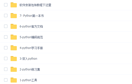
三、全套PDF电子书

书籍的好处就在于权威和体系健全，刚开始学习的时候你可以只看视频或者听某个人讲课，但等你学完之后，你觉得你掌握了，这时候建议还是得去看一下书籍，看权威技术书籍也是每个程序员必经之路。

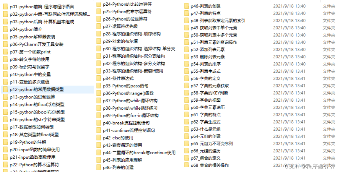
四、入门学习视频

我们在看视频学习的时候，不能光动眼动脑不动手，比较科学的学习方法是在理解之后运用它们，这时候练手项目就很适合了。

五、实战案例

光学理论是没用的，要学会跟着一起敲，要动手实操，才能将自己的所学运用到实际当中去，这时候可以搞点实战案例来学习。

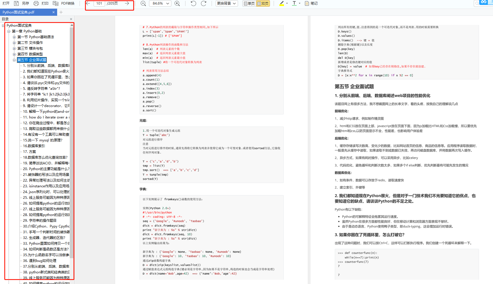
六、面试资料

我们学习Python必然是为了找到高薪的工作，下面这些面试题是来自阿里、腾讯、字节等一线互联网大厂最新的面试资料，并且有阿里大佬给出了权威的解答，刷完这一套面试资料相信大家都能找到满意的工作。

网上学习资料一大堆，但如果学到的知识不成体系，遇到问题时只是浅尝辄止，不再深入研究，那么很难做到真正的技术提升。

需要这份系统化学习资料的朋友，可以戳这里获取

一个人可以走的很快，但一群人才能走的更远！不论你是正从事IT行业的老鸟或是对IT行业感兴趣的新人，都欢迎加入我们的的圈子（技术交流、学习资源、职场吐槽、大厂内推、面试辅导），让我们一起学习成长！