永磁同步电机无位置传感器控制技术之高频正弦波注入-----旋转高频注入法（理论推导）

旋转的电机

已于 2024-03-15 10:57:41 修改

阅读量759

点赞数 8

文章标签：单片机嵌入式硬件

于 2024-03-14 20:56:01 首次发布

本文链接：https://blog.csdn.net/m0_62155925/article/details/136707506

版权

本文详细讨论了永磁同步电机在低速下的数学模型，重点介绍了坐标变换、高频响应电流计算以及利用外差法提取转子位置的方法。通过简单的外差法处理，结合低通滤波器，最终实现转子位置的估计。

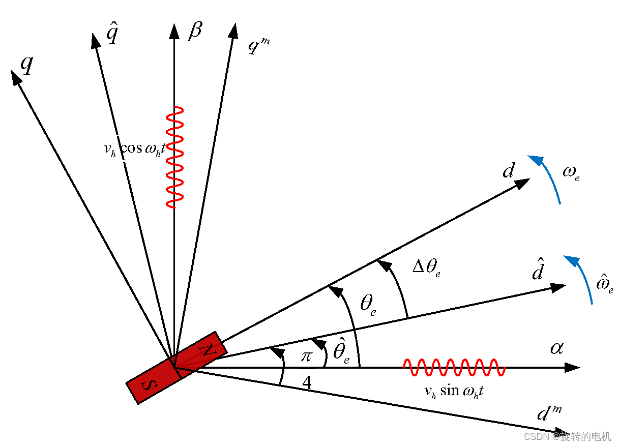
摘要由CSDN通过智能技术生成

图1 几种坐标系关系

永磁同步迪电机在零低速下数学模型可以看成一个纯电感模型（忽略反电势（反电势信噪比低，占比低）、电阻压降（在高频信号激励下，电阻压降占比远小于电感压降））

$\left[ {\begin{array}{*{20}{c}} {{u_{dh}}}\\ {{u_{qh}}} \end{array}} \right] = \left[ {\begin{array}{*{20}{c}} {{L_d}}&0\\ 0&{{L_q}} \end{array}} \right]\left[ {\begin{array}{*{20}{c}} {p{i_{dh}}}\\ {p{i_{qh}}} \end{array}} \right]$ （1）

定义坐标变换

$T(\theta ) = \left[ {\begin{array}{*{20}{c}} {\cos (\theta )}&{\sin (\theta )}\\ { - \sin (\theta )}&{\cos (\theta )} \end{array}} \right]$ （2）

注：逆时针旋转，相当于左乘一个 $T(\theta )$ 矩阵；顺时针旋转，相当于相当于左乘一个 ${T^{ - 1}}(\theta )$ 矩阵。

$d-q$ 坐标系顺时针旋转 $\theta_{e}$ 角度到 $\alpha-\beta$ 坐标系，对于电压，则有 $\begin{array}{l} \left[ {\begin{array}{*{20}{c}} {{u_{\alpha h}}}\\ {{u_{\beta h}}} \end{array}} \right] = {T^{ - 1}}\left( {{\theta _e}} \right)\left[ {\begin{array}{*{20}{c}} {{u_{dh}}}\\ {{u_{qh}}} \end{array}} \right] = \left[ {\begin{array}{*{20}{c}} {\cos ({\theta _e})}&{ - \sin ({\theta _e})}\\ {\sin ({\theta _e})}&{\cos ({\theta _e})} \end{array}} \right]\left[ {\begin{array}{*{20}{c}} {{L_d}}&0\\ 0&{{L_q}} \end{array}} \right]\left[ {\begin{array}{*{20}{c}} {p{i_{dh}}}\\ {p{i_{qh}}} \end{array}} \right]\\ = \left[ {\begin{array}{*{20}{c}} {\frac{{{L_d} + {L_q}}}{2} + \frac{{{L_d} - {L_q}}}{2}\cos (2{\theta _e})}&{\frac{{{L_d} - {L_q}}}{2}\sin (2{\theta _e})}\\ {\frac{{{L_d} - {L_q}}}{2}\sin (2{\theta _e})}&{\frac{{{L_d} + {L_q}}}{2} - \frac{{{L_d} - {L_q}}}{2}\cos (2{\theta _e})} \end{array}} \right]\\ = \left[ {\begin{array}{*{20}{c}} {{L_\Sigma } + {L_\Delta }\cos (2{\theta _e})}&{{L_\Delta }\sin (2{\theta _e})}\\ {{L_\Delta }\sin (2{\theta _e})}&{{L_\Sigma } - {L_\Delta }\cos (2{\theta _e})} \end{array}} \right]\left[ {\begin{array}{*{20}{c}} {p{i_{\alpha h}}}\\ {p{i_{\beta h}}} \end{array}} \right] \end{array}$ (3)

式（3）中， ${L_\Sigma } = \frac{{{L_d} + {L_q}}}{2}$ ， ${L_\Delta } = \frac{{{L_d} - {L_q}}}{2}$ 。

则式（3）可以变为

$\left[ {\begin{array}{*{20}{c}} {p{i_{\alpha h}}}\\ {p{i_{\beta h}}} \end{array}} \right] = {\left[ {\begin{array}{*{20}{c}} {{L_\Sigma } + {L_\Delta }\cos (2{\theta _e})}&{{L_\Delta }\sin (2{\theta _e})}\\ {{L_\Delta }\sin (2{\theta _e})}&{{L_\Sigma } - {L_\Delta }\cos (2{\theta _e})} \end{array}} \right]^{ - 1}}\left[ {\begin{array}{*{20}{c}} {{u_{\alpha h}}}\\ {{u_{\beta h}}} \end{array}} \right]$ （4）

注入的正弦波形式为

$\left[ {\begin{array}{*{20}{c}} {{u_{\alpha h}}}\\ {{u_{\beta h}}} \end{array}} \right] = {v_h}\left[ {\begin{array}{*{20}{c}} {\cos ({\omega _h}t)}\\ {\sin ({\omega _h}t)} \end{array}} \right]$ （5）

将式（5）带入式（4）可得则 $\alpha-\beta$ 坐标系下高频响应电流为

$\begin{array}{l} \left[ {\begin{array}{*{20}{c}} {{i_{\alpha h}}}\\ {{i_{\beta h}}} \end{array}} \right] = {\left[ {\begin{array}{*{20}{c}} {{L_\Sigma } + {L_\Delta }\cos (2{\theta _e})}&{{L_\Delta }\sin (2{\theta _e})}\\ {{L_\Delta }\sin (2{\theta _e})}&{{L_\Sigma } - {L_\Delta }\cos (2{\theta _e})} \end{array}} \right]^{ - 1}}\int {\left[ {\begin{array}{*{20}{c}} {{u_{\alpha h}}}\\ {{u_{\beta h}}} \end{array}} \right]} \\ = K\left[ {\begin{array}{*{20}{c}} {{L_\Sigma }\sin ({\omega _h}t) + {L_\Delta }\sin (2{\theta _e} - {\omega _h}t)}\\ { - {L_\Sigma }\cos ({\omega _h}t) - {L_\Delta }\cos (2{\theta _e} - {\omega _h}t)} \end{array}} \right] \end{array}$ （6）

式（6）中， $K=\frac{{{v_h}}}{{{\omega _h}(L_\Sigma ^2 - L_\Delta ^2)}}$ 。接下来需要从高频响应电流中提取出角度 $\theta_{e}$ ，本文采取较为简单的外差法解耦转子位置（不采用同步轴系滤波器，太复杂，容易绕晕），如图2所示。

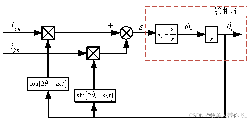
图2 外差法转子位置提取法

$\begin{array}{l} {i_{\alpha h}}.\cos (2{{\hat \theta }_e} - {\omega _h}t) + {i_{\beta h}}.\sin (2{{\hat \theta }_e} - {\omega _h}t)\\ = K{L_\Sigma }\sin (2{\omega _h}t - 2{{\hat \theta }_e}) + K{L_\Delta }\sin (2{\theta _e} - 2{{\hat \theta }_e}) \end{array}$ （7）