


國值分割练习题
对红细胞图像cell1.jpg实现阈值分割
1:绘制直方图,根据直方图,设置不同阈值观察效果,选择合适的阈值
2:利用OSTU法实现分割
3:利用均值自适应,高斯自适应分割
4:写程序实现OSTU算法
阈值的选择直接影响分割效果,通常可以分析图像的灰度直方图来确定最佳阈值
利用灰度直方图求双峰或多峰中两峰之间的谷底作为值,分割效果较好。
### 1:绘制直方图,根据直方图,设置不同阈值观察效果,选择合适的阈值
import cv2
import numpy as np
from matplotlib import pyplot as plt

# 读取图像
img = cv2.imread('image/cell1.jpg',0)

# 计算直方图
hist = cv2.calcHist([img],[0],None,[256],[0,256])

# 绘制直方图
plt.figure(figsize=(5,4))
plt.title("Grayscale Histogram")
plt.xlabel("Bins")
plt.ylabel("# of Pixels")

# 使用fill_between来填充曲线下的区域
plt.fill_between(range(256), hist.flatten(), color='#1F77B4')

# 设置x轴和y轴的限制
plt.xlim([0, 256])
plt.ylim([0, max(hist)])

plt.show()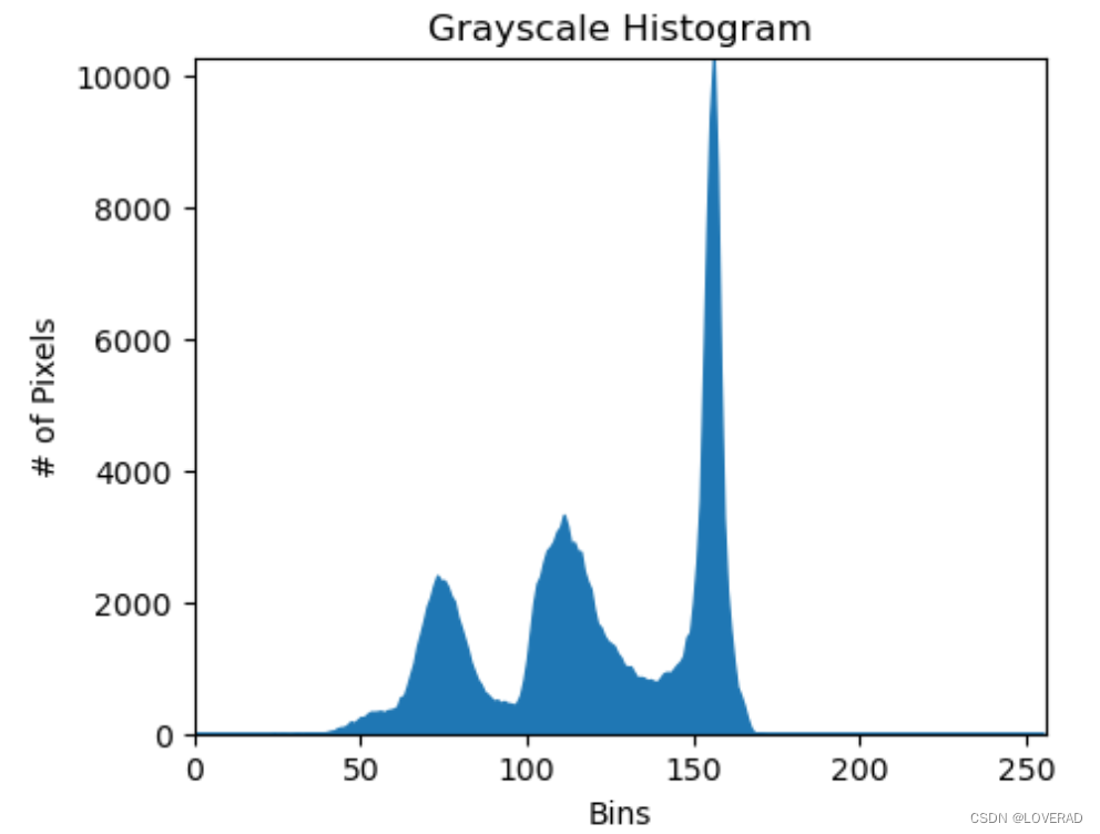
# 设置不同的阈值
thresholds = [75, 95, 115, 135, 155]

# 创建一个新的figure
plt.figure(figsize=(10,6))

# 在第一个位置显示原图
plt.subplot(2,3,1)
plt.title("Original Image")
plt.imshow(img, cmap='gray')

# 对每个阈值应用阈值分割,并在subplot中显示结果
for i, thresh in enumerate(thresholds):
    # 应用阈值
    ret,thresh_img = cv2.threshold(img,thresh,255,cv2.THRESH_BINARY)

    # 绘制阈值图像
    plt.subplot(2,3,i+2)
    plt.title(f"Thresh = {thresh}")
    plt.imshow(thresh_img, cmap='gray')

# 显示所有的图像
plt.show()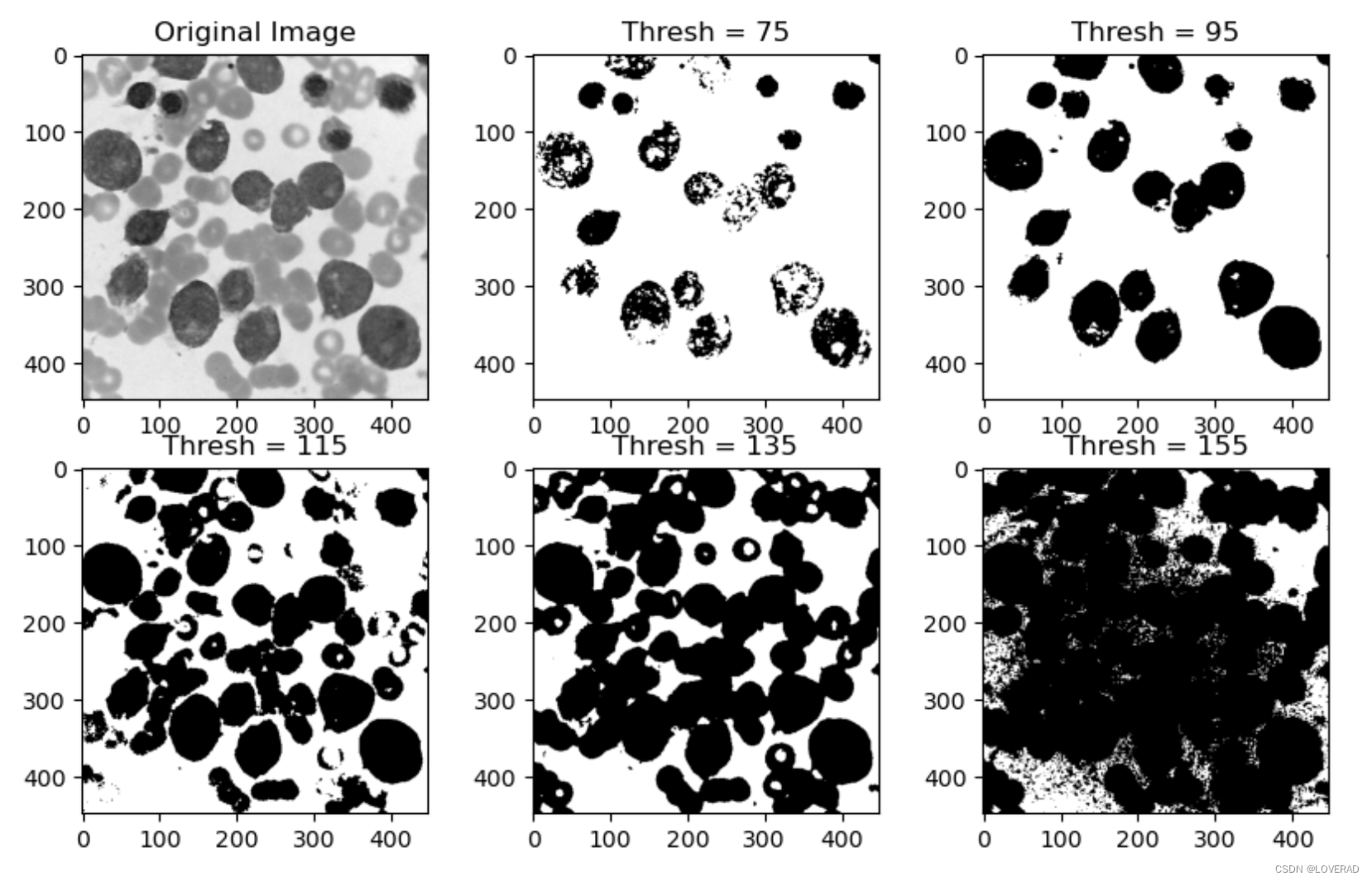
### 2:利用OSTU法实现分割
# 读取图像
img = cv2.imread('image/cell1.jpg',0)

# 使用OSTU阈值方法进行阈值分割
ret, thresh = cv2.threshold(img, 0, 255, cv2.THRESH_BINARY + cv2.THRESH_OTSU)

# 显示图像
plt.figure(figsize=(5,4))
plt.title("Image after OSTU thresholding")
plt.imshow(thresh, cmap='gray')
plt.show()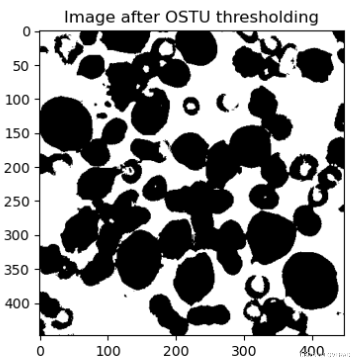
### 3:利用均值自适应,高斯自适应分割
img = cv2.imread('image/cell1.jpg',0)

# 使用均值自适应阈值分割
mean_thresh = cv2.adaptiveThreshold(img, 255, cv2.ADAPTIVE_THRESH_MEAN_C, cv2.THRESH_BINARY, 11, 2)

# 使用高斯自适应阈值分割
gaussian_thresh = cv2.adaptiveThreshold(img, 255, cv2.ADAPTIVE_THRESH_GAUSSIAN_C, cv2.THRESH_BINARY, 11, 2)

# 显示图像
plt.figure(figsize=(10,4))

plt.subplot(1,2,1)
plt.title("Image after Mean Adaptive Thresholding")
plt.imshow(mean_thresh, cmap='gray')

plt.subplot(1,2,2)
plt.title("Image after Gaussian Adaptive Thresholding")
plt.imshow(gaussian_thresh, cmap='gray')

plt.show()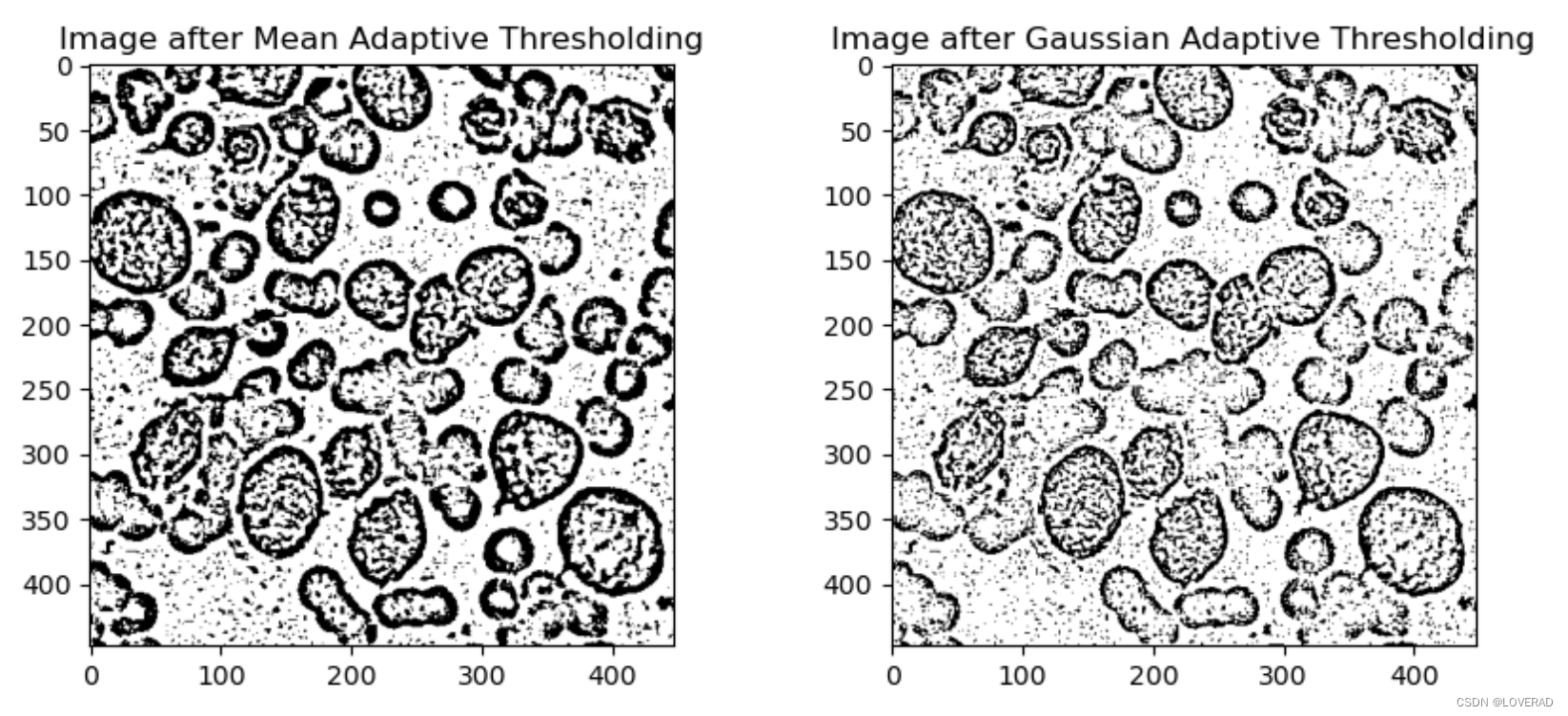
### 4:写程序实现OSTU算法
# 读取图像
img = cv2.imread('image/cell1.jpg',0)

# 计算直方图
hist = cv2.calcHist([img],[0],None,[256],[0,256])

# 归一化直方图
hist_norm = hist.ravel()/hist.max()
Q = hist_norm.cumsum()

bins = np.arange(256)

fn_min = np.inf
thresh = -1
# 相当于手动实现了cv2.THRESH_OTSU
for i in range(1,256):
    p1,p2 = np.hsplit(hist_norm,[i]) # 概率
    q1,q2 = Q[i],Q[255]-Q[i] # 累积概率
    if q1 < 1.e-6 or q2 < 1.e-6:
        continue
    m1,m2 = np.sum(p1*bins[:i])/q1, np.sum(p2*bins[i:])/q2 # 均值
    v1,v2 = np.sum(((bins[:i]-m1)**2)*p1)/q1,np.sum(((bins[i:]-m2)**2)*p2)/q2 # 方差

    # 计算最小化函数
    fn = v1*q1 + v2*q2
    if fn < fn_min:
        fn_min = fn
        thresh = i

# 使用Otsu的阈值进行阈值分割
ret, otsu = cv2.threshold(img, thresh, 255, cv2.THRESH_BINARY)

# 显示图像
plt.figure(figsize=(5,4))
plt.title("Image after manual OSTU thresholding")
plt.imshow(otsu, cmap='gray')
plt.show()

print(f'Otsu  thresholding value : {thresh}')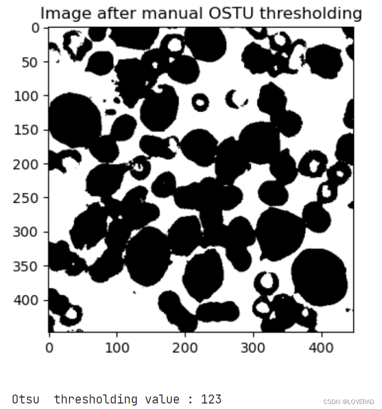


 7万+
7万+

 被折叠的 条评论
为什么被折叠?
被折叠的 条评论
为什么被折叠?
 到【灌水乐园】发言


