Spl-kan&Wav-kan代码概览overlook

目录

KANlayer

类定义和初始化

属性

网格和系数

可训练与不可训练的识别

初始化噪声和掩码

基函数和尺度

前向传播

解释：

具体实现

其他方法

wav-kan

类定义和初始化

小波变换方法

参数在这里

可学习的参数（Learnable Parameters）：

不可学习的参数（Non-Learnable Parameters）：

前向传播方法

KAN 类

总结

一般性的

---

KANlayer

 https://github.com/KindXiaoming/pykan#start-of-content

import torch
import torch.nn as nn
import numpy as np
from .spline import *
from .utils import sparse_mask


class KANLayer(nn.Module):
    """
    KANLayer class
    

    Attributes:
    -----------
        in_dim: int
            input dimension
        out_dim: int
            output dimension
        num: int
            the number of grid intervals
        k: int
            the piecewise polynomial order of splines
        noise_scale: float
            spline scale at initialization
        coef: 2D torch.tensor
            coefficients of B-spline bases
        scale_base_mu: float
            magnitude of the residual function b(x) is drawn from N(mu, sigma^2), mu = sigma_base_mu
        scale_base_sigma: float
            magnitude of the residual function b(x) is drawn from N(mu, sigma^2), mu = sigma_base_sigma
        scale_sp: float
            mangitude of the spline function spline(x)
        base_fun: fun
            residual function b(x)
        mask: 1D torch.float
            mask of spline functions. setting some element of the mask to zero means setting the corresponding activation to zero function.
        grid_eps: float in [0,1]
            a hyperparameter used in update_grid_from_samples. When grid_eps = 1, the grid is uniform; when grid_eps = 0, the grid is partitioned using percentiles of samples. 0 < grid_eps < 1 interpolates between the two extremes.
            the id of activation functions that are locked
        device: str
            device
    """

    def __init__(self, in_dim=3, out_dim=2, num=5, k=3, noise_scale=0.5, scale_base_mu=0.0, scale_base_sigma=1.0, scale_sp=1.0, base_fun=torch.nn.SiLU(), grid_eps=0.02, grid_range=[-1, 1], sp_trainable=True, sb_trainable=True, save_plot_data = True, device='cpu', sparse_init=False):
        ''''
        initialize a KANLayer
        
        Args:
        -----
            in_dim : int
                input dimension. Default: 2.
            out_dim : int
                output dimension. Default: 3.
            num : int
                the number of grid intervals = G. Default: 5.
            k : int
                the order of piecewise polynomial. Default: 3.
            noise_scale : float
                the scale of noise injected at initialization. Default: 0.1.
            scale_base_mu : float
                the scale of the residual function b(x) is intialized to be N(scale_base_mu, scale_base_sigma^2).
            scale_base_sigma : float
                the scale of the residual function b(x) is intialized to be N(scale_base_mu, scale_base_sigma^2).
            scale_sp : float
                the scale of the base function spline(x).
            base_fun : function
                residual function b(x). Default: torch.nn.SiLU()
            grid_eps : float
                When grid_eps = 1, the grid is uniform; when grid_eps = 0, the grid is partitioned using percentiles of samples. 0 < grid_eps < 1 interpolates between the two extremes.
            grid_range : list/np.array of shape (2,)
                setting the range of grids. Default: [-1,1].
            sp_trainable : bool
                If true, scale_sp is trainable
            sb_trainable : bool
                If true, scale_base is trainable
            device : str
                device
            sparse_init : bool
                if sparse_init = True, sparse initialization is applied.
            
        Returns:
        --------
            self
            
        Example
        -------
        >>> from kan.KANLayer import *
        >>> model = KANLayer(in_dim=3, out_dim=5)
        >>> (model.in_dim, model.out_dim)
        '''
        super(KANLayer, self).__init__()
        # size 
        self.out_dim = out_dim
        self.in_dim = in_dim
        self.num = num
        self.k = k

        grid = torch.linspace(grid_range[0], grid_range[1], steps=num + 1)[None,:].expand(self.in_dim, num+1)
        grid = extend_grid(grid, k_extend=k)
        self.grid = torch.nn.Parameter(grid).requires_grad_(False)
        noises = (torch.rand(self.num+1, self.in_dim, self.out_dim) - 1/2) * noise_scale / num

        self.coef = torch.nn.Parameter(curve2coef(self.grid[:,k:-k].permute(1,0), noises, self.grid, k))
        
        if sparse_init:
            self.mask = torch.nn.Parameter(sparse_mask(in_dim, out_dim)).requires_grad_(False)
        else:
            self.mask = torch.nn.Parameter(torch.ones(in_dim, out_dim)).requires_grad_(False)
        
        self.scale_base = torch.nn.Parameter(scale_base_mu * 1 / np.sqrt(in_dim) + \
                         scale_base_sigma * (torch.rand(in_dim, out_dim)*2-1) * 1/np.sqrt(in_dim)).requires_grad_(sb_trainable)
        self.scale_sp = torch.nn.Parameter(torch.ones(in_dim, out_dim) * scale_sp * 1 / np.sqrt(in_dim) * self.mask).requires_grad_(sp_trainable)  # make scale trainable
        self.base_fun = base_fun

        
        self.grid_eps = grid_eps
        
        self.to(device)
        
    def to(self, device):
        super(KANLayer, self).to(device)
        self.device = device    
        return self

    def forward(self, x):
        '''
        KANLayer forward given input x
        
        Args:
        -----
            x : 2D torch.float
                inputs, shape (number of samples, input dimension)
            
        Returns:
        --------
            y : 2D torch.float
                outputs, shape (number of samples, output dimension)
            preacts : 3D torch.float
                fan out x into activations, shape (number of sampels, output dimension, input dimension)
            postacts : 3D torch.float
                the outputs of activation functions with preacts as inputs
            postspline : 3D torch.float
                the outputs of spline functions with preacts as inputs
        
        Example
        -------
        >>> from kan.KANLayer import *
        >>> model = KANLayer(in_dim=3, out_dim=5)
        >>> x = torch.normal(0,1,size=(100,3))
        >>> y, preacts, postacts, postspline = model(x)
        >>> y.shape, preacts.shape, postacts.shape, postspline.shape
        '''
        batch = x.shape[0]
        preacts = x[:,None,:].clone().expand(batch, self.out_dim, self.in_dim)
            
        base = self.base_fun(x) # (batch, in_dim)
        y = coef2curve(x_eval=x, grid=self.grid, coef=self.coef, k=self.k)
        
        postspline = y.clone().permute(0,2,1)
            
        y = self.scale_base[None,:,:] * base[:,:,None] + self.scale_sp[None,:,:] * y
        y = self.mask[None,:,:] * y
        
        postacts = y.clone().permute(0,2,1)
            
        y = torch.sum(y, dim=1)
        return y, preacts, postacts, postspline

    def update_grid_from_samples(self, x, mode='sample'):
        '''
        update grid from samples
        
        Args:
        -----
            x : 2D torch.float
                inputs, shape (number of samples, input dimension)
            
        Returns:
        --------
            None
        
        Example
        -------
        >>> model = KANLayer(in_dim=1, out_dim=1, num=5, k=3)
        >>> print(model.grid.data)
        >>> x = torch.linspace(-3,3,steps=100)[:,None]
        >>> model.update_grid_from_samples(x)
        >>> print(model.grid.data)
        '''
        
        batch = x.shape[0]
        #x = torch.einsum('ij,k->ikj', x, torch.ones(self.out_dim, ).to(self.device)).reshape(batch, self.size).permute(1, 0)
        x_pos = torch.sort(x, dim=0)[0]
        y_eval = coef2curve(x_pos, self.grid, self.coef, self.k)
        num_interval = self.grid.shape[1] - 1 - 2*self.k
        
        def get_grid(num_interval):
            ids = [int(batch / num_interval * i) for i in range(num_interval)] + [-1]
            grid_adaptive = x_pos[ids, :].permute(1,0)
            margin = 0.00
            h = (grid_adaptive[:,[-1]] - grid_adaptive[:,[0]] + 2 * margin)/num_interval
            grid_uniform = grid_adaptive[:,[0]] - margin + h * torch.arange(num_interval+1,)[None, :].to(x.device)
            grid = self.grid_eps * grid_uniform + (1 - self.grid_eps) * grid_adaptive
            return grid
        
        
        grid = get_grid(num_interval)
        
        if mode == 'grid':
            sample_grid = get_grid(2*num_interval)
            x_pos = sample_grid.permute(1,0)
            y_eval = coef2curve(x_pos, self.grid, self.coef, self.k)
        
        self.grid.data = extend_grid(grid, k_extend=self.k)
        #print('x_pos 2', x_pos.shape)
        #print('y_eval 2', y_eval.shape)
        self.coef.data = curve2coef(x_pos, y_eval, self.grid, self.k)

    def initialize_grid_from_parent(self, parent, x, mode='sample'):
        '''
        update grid from a parent KANLayer & samples
        
        Args:
        -----
            parent : KANLayer
                a parent KANLayer (whose grid is usually coarser than the current model)
            x : 2D torch.float
                inputs, shape (number of samples, input dimension)
            
        Returns:
        --------
            None
          
        Example
        -------
        >>> batch = 100
        >>> parent_model = KANLayer(in_dim=1, out_dim=1, num=5, k=3)
        >>> print(parent_model.grid.data)
        >>> model = KANLayer(in_dim=1, out_dim=1, num=10, k=3)
        >>> x = torch.normal(0,1,size=(batch, 1))
        >>> model.initialize_grid_from_parent(parent_model, x)
        >>> print(model.grid.data)
        '''
        
        batch = x.shape[0]
        
        # shrink grid
        x_pos = torch.sort(x, dim=0)[0]
        y_eval = coef2curve(x_pos, parent.grid, parent.coef, parent.k)
        num_interval = self.grid.shape[1] - 1 - 2*self.k
        
        
        '''
        # based on samples
        def get_grid(num_interval):
            ids = [int(batch / num_interval * i) for i in range(num_interval)] + [-1]
            grid_adaptive = x_pos[ids, :].permute(1,0)
            h = (grid_adaptive[:,[-1]] - grid_adaptive[:,[0]])/num_interval
            grid_uniform = grid_adaptive[:,[0]] + h * torch.arange(num_interval+1,)[None, :].to(x.device)
            grid = self.grid_eps * grid_uniform + (1 - self.grid_eps) * grid_adaptive
            return grid'''
        
        #print('p', parent.grid)
        # based on interpolating parent grid
        def get_grid(num_interval):
            x_pos = parent.grid[:,parent.k:-parent.k]
            #print('x_pos', x_pos)
            sp2 = KANLayer(in_dim=1, out_dim=self.in_dim,k=1,num=x_pos.shape[1]-1,scale_base_mu=0.0, scale_base_sigma=0.0).to(x.device)

            #print('sp2_grid', sp2.grid[:,sp2.k:-sp2.k].permute(1,0).expand(-1,self.in_dim))
            #print('sp2_coef_shape', sp2.coef.shape)
            sp2_coef = curve2coef(sp2.grid[:,sp2.k:-sp2.k].permute(1,0).expand(-1,self.in_dim), x_pos.permute(1,0).unsqueeze(dim=2), sp2.grid[:,:], k=1).permute(1,0,2)
            shp = sp2_coef.shape
            #sp2_coef = torch.cat([torch.zeros(shp[0], shp[1], 1), sp2_coef, torch.zeros(shp[0], shp[1], 1)], dim=2)
            #print('sp2_coef',sp2_coef)
            #print(sp2.coef.shape)
            sp2.coef.data = sp2_coef
            percentile = torch.linspace(-1,1,self.num+1).to(self.device)
            grid = sp2(percentile.unsqueeze(dim=1))[0].permute(1,0)
            #print('c', grid)
            return grid
        
        grid = get_grid(num_interval)
        
        if mode == 'grid':
            sample_grid = get_grid(2*num_interval)
            x_pos = sample_grid.permute(1,0)
            y_eval = coef2curve(x_pos, parent.grid, parent.coef, parent.k)
        
        grid = extend_grid(grid, k_extend=self.k)
        self.grid.data = grid
        self.coef.data = curve2coef(x_pos, y_eval, self.grid, self.k)

    def get_subset(self, in_id, out_id):
        '''
        get a smaller KANLayer from a larger KANLayer (used for pruning)
        
        Args:
        -----
            in_id : list
                id of selected input neurons
            out_id : list
                id of selected output neurons
            
        Returns:
        --------
            spb : KANLayer
            
        Example
        -------
        >>> kanlayer_large = KANLayer(in_dim=10, out_dim=10, num=5, k=3)
        >>> kanlayer_small = kanlayer_large.get_subset([0,9],[1,2,3])
        >>> kanlayer_small.in_dim, kanlayer_small.out_dim
        (2, 3)
        '''
        spb = KANLayer(len(in_id), len(out_id), self.num, self.k, base_fun=self.base_fun)
        spb.grid.data = self.grid[in_id]
        spb.coef.data = self.coef[in_id][:,out_id]
        spb.scale_base.data = self.scale_base[in_id][:,out_id]
        spb.scale_sp.data = self.scale_sp[in_id][:,out_id]
        spb.mask.data = self.mask[in_id][:,out_id]

        spb.in_dim = len(in_id)
        spb.out_dim = len(out_id)
        return spb
    
    
    def swap(self, i1, i2, mode='in'):
        '''
        swap the i1 neuron with the i2 neuron in input (if mode == 'in') or output (if mode == 'out') 
        
        Args:
        -----
            i1 : int
            i2 : int
            mode : str
                mode = 'in' or 'out'
            
        Returns:
        --------
            None
            
        Example
        -------
        >>> from kan.KANLayer import *
        >>> model = KANLayer(in_dim=2, out_dim=2, num=5, k=3)
        >>> print(model.coef)
        >>> model.swap(0,1,mode='in')
        >>> print(model.coef)
        '''
        with torch.no_grad():
            def swap_(data, i1, i2, mode='in'):
                if mode == 'in':
                    data[i1], data[i2] = data[i2].clone(), data[i1].clone()
                elif mode == 'out':
                    data[:,i1], data[:,i2] = data[:,i2].clone(), data[:,i1].clone()

            if mode == 'in':
                swap_(self.grid.data, i1, i2, mode='in')
            swap_(self.coef.data, i1, i2, mode=mode)
            swap_(self.scale_base.data, i1, i2, mode=mode)
            swap_(self.scale_sp.data, i1, i2, mode=mode)
            swap_(self.mask.data, i1, i2, mode=mode)

这段代码定义了一个名为 KANLayer 的 PyTorch 模块，它实现了一种特殊的神经网络层，称为 Kolmogorov-Arnold Networks（KAN）层。以下是代码的详细解释：

类定义和初始化

class KANLayer(nn.Module):
    ...
    def __init__(self, in_dim=3, out_dim=2, num=5, k=3, noise_scale=0.5, ...):
        super(KANLayer, self).__init__()
        ...

• KANLayer 继承自 nn.Module，是 PyTorch 中的一个自定义层。
• 初始化方法 __init__ 接受多个参数，包括输入维度 in_dim、输出维度 out_dim、网格间隔数 num、多项式阶数 k、初始化噪声尺度 noise_scale 等。

属性

self.out_dim = out_dim
self.in_dim = in_dim
self.num = num
self.k = k
...

• 这些属性保存了层的配置参数。

网格和系数

grid = torch.linspace(grid_range[0], grid_range[1], steps=num + 1)[None,:].expand(self.in_dim, num+1)
grid = extend_grid(grid, k_extend=k)
self.grid = torch.nn.Parameter(grid).requires_grad_(False)
...
self.coef = torch.nn.Parameter(curve2coef(self.grid[:,k:-k].permute(1,0), noises, self.grid, k))

• 创建一个网格 grid，它定义了 B-样条基函数的位置。
• extend_grid 可能是一个扩展网格以包含更高阶多项式的函数。
• self.grid 是一个不可训练的参数。
• self.coef 是 B-样条基函数的系数，是可训练的参数。

可训练与不可训练的识别

从代码中可以看出，self.grid 被设置为不可训练的参数，因为它在初始化时被设置了 requires_grad_(False)。这意味着在训练过程中，self.grid 的值不会随着反向传播而更新。

相反，self.coef 被设置为可训练的参数，因为它在初始化时被设置了 requires_grad_(True)。这意味着在训练过程中，self.coef 的值会随着反向传播而更新，从而允许网络学习优化这些参数。

具体来说，代码中如下所示：

self.grid = torch.nn.Parameter(grid).requires_grad_(False)
self.coef = torch.nn.Parameter(curve2coef(self.grid[:,k:-k].permute(1,0), noises, self.grid, k))

这里，self.grid 被初始化为 grid，并且设置为不可训练。而 self.coef 则是通过 curve2coef 函数计算得出的，并且设置为可训练。

初始化噪声和掩码

noises = (torch.rand(self.num+1, self.in_dim, self.out_dim) - 1/2) * noise_scale / num
...
if sparse_init:
    self.mask = torch.nn.Parameter(sparse_mask(in_dim, out_dim)).requires_grad_(False)
else:
    self.mask = torch.nn.Parameter(torch.ones(in_dim, out_dim)).requires_grad_(False)

• 初始化噪声 noises 用于生成 B-样条系数的初始值。
• self.mask 是一个掩码，用于控制哪些激活函数是活动的（非零），默认情况下所有激活函数都是活动的。

基函数和尺度

self.scale_base = torch.nn.Parameter(...)
self.scale_sp = torch.nn.Parameter(...)
self.base_fun = base_fun

• self.scale_base 和 self.scale_sp 是可训练的参数，用于调整基函数和残差函数的尺度。
• self.base_fun 是一个激活函数，默认为 SiLU。

前向传播

def forward(self, x):
    ...
    return y, preacts, postacts, postspline

解释：

总的来说，这段注释描述了神经网络层在前向传播过程中涉及的不同类型的张量及其维度，包括线性组合的结果（预激活值）、激活函数的输出以及样条函数的输出。

具体实现

• forward 方法实现了层的前向传播。
• 输入 x 通过 B-样条基函数和残差函数进行处理，生成输出 y。
• 返回值包括输出 y、预激活 preacts、后激活 postacts 和 B-样条函数的输出 postspline。
• y: 2D torch.float
  • 输出，形状为（样本数量，输出维度）
• preacts: 3D torch.float
  • 从输入到激活的扇出，形状为（样本数量，输出维度，输入维度）
• postacts: 3D torch.float
  • 以 preacts 作为输入的激活函数的输出
• postspline: 3D torch.float
  • 以 preacts 作为输入的样条函数的输出
• y: 这是一个二维张量，表示神经网络的输出。其中，第一个维度代表样本的数量，第二个维度代表每个样本的输出维度。
• preacts: 这是一个三维张量，表示在激活函数之前，每个输出神经元对输入数据的线性组合（即预激活值）。第一个维度代表样本数量，第二个维度代表输出维度（即神经元的数量），第三个维度代表输入维度（即每个样本的特征数量）。
• postacts: 这也
• 是一个三维张量，它包含了 preacts 经过激活函数处理后的结果。每个输出神经元的激活值是基于其对应的预激活值计算得出的。
• postspline: 这同样是一个三维张量，它表示 preacts 经过样条函数处理后的输出。样条函数可能是网络中的一个非线性处理步骤，用于生成更加复杂的特征表示。

这段代码是 KANLayer 类中 forward 方法的实现，它定义了神经网络层的前向传播过程。以下是对代码的详细解释：

batch = x.shape[0]

这行代码获取输入数据 x 的批次大小（即样本数量）。

preacts = x[:,None,:].clone().expand(batch, self.out_dim, self.in_dim)

base = self.base_fun(x) # (batch, in_dim)

y = coef2curve(x_eval=x, grid=self.grid, coef=self.coef, k=self.k)

postspline = y.clone().permute(0,2,1)

y = self.scale_base[None,:,:] * base[:,:,None] + self.scale_sp[None,:,:] * y

y = self.mask[None,:,:] * y

postacts = y.clone().permute(0,2,1)

y = torch.sum(y, dim=1)

复制

return y, preacts, postacts, postspline

这个 forward 方法展示了如何将输入数据 x 通过一个复杂的神经网络层进行处理，包括线性组合、样条函数的应用、激活、加权以及掩码操作。

python

• x[:,None,:] 将输入 x 的形状从 (batch, in_dim) 变为 (batch, 1, in_dim)，通过在中间插入一个维度。
• .clone() 创建了这个新形状的张量的一个副本。
• .expand(batch, self.out_dim, self.in_dim) 将这个副本扩展到新的形状 (batch, out_dim, in_dim)，其中 out_dim 是输出维度。这样，每个输入样本都被复制了 out_dim 次，以便与每个输出神经元对应。
• 这行代码应用了一个基础函数 base_fun 到输入 x 上，该函数的输出形状为 (batch, in_dim)。
• coef2curve 函数根据给定的网格 grid、系数 coef 和样条度数 k，计算样条曲线的值。x_eval 是要评估样条曲线的点，这里使用输入 x。
• .clone() 创建了 y 的一个副本。
• .permute(0,2,1) 改变了张量的维度顺序，从 (batch, out_dim, in_dim) 变为 (batch, in_dim, out_dim)。
• self.scale_base[None,:,:] 和 self.scale_sp[None,:,:] 分别是将 scale_base 和 scale_sp 张量添加一个批次维度。
• 这行代码计算了基于基础函数和样条函数的加权组合。
• 这行代码应用了一个掩码 mask 到 y 上，可能是用于稀疏化或特定特征的屏蔽。
• 与 postspline 类似，这行代码创建了 y 的一个副本，并改变了其维度顺序。
• 这行代码对 y 在第二个维度（输出维度）上进行求和，从而得到每个样本的最终输出。
• 最后，方法返回了四个张量：y（输出），preacts（预激活值），postacts（激活后的输出），和 postspline（样条函数的输出）。

其他方法

• to(device): 将层移到指定设备。
• update_grid_from_samples(x, mode='sample'): 根据样本 x 更新网格。
• initialize_grid_from_parent(parent, x, mode='sample'): 从父层和样本 x 初始化网格。
• get_subset(in_id, out_id): 获取层的子集，用于剪枝。
• swap(i1, i2, mode='in'): 交换输入或输出神经元。

这段代码展示了如何定义一个复杂的神经网络层，其中包含了网格的初始化、系数的学习、以及如何处理输入以生成输出。这种类型的层可以用于学习复杂的函数表示。

将B spline融入forward前向传播。

wav-kan

https://github.com/zavareh1/Wav-KAN/blob/main/README.md

'''This is a sample code for the simulations of the paper:
Bozorgasl, Zavareh and Chen, Hao, Wav-KAN: Wavelet Kolmogorov-Arnold Networks (May, 2024)

https://arxiv.org/abs/2405.12832
and also available at:
https://papers.ssrn.com/sol3/papers.cfm?abstract_id=4835325
We used efficient KAN notation and some part of the code:https://github.com/Blealtan/efficient-kan

'''
import torch
import torch.nn as nn
import torch.nn.functional as F
import torch.optim as optim
import torchvision
import torchvision.transforms as transforms
from torch.utils.data import DataLoader
from tqdm import tqdm
import math

class KANLinear(nn.Module):
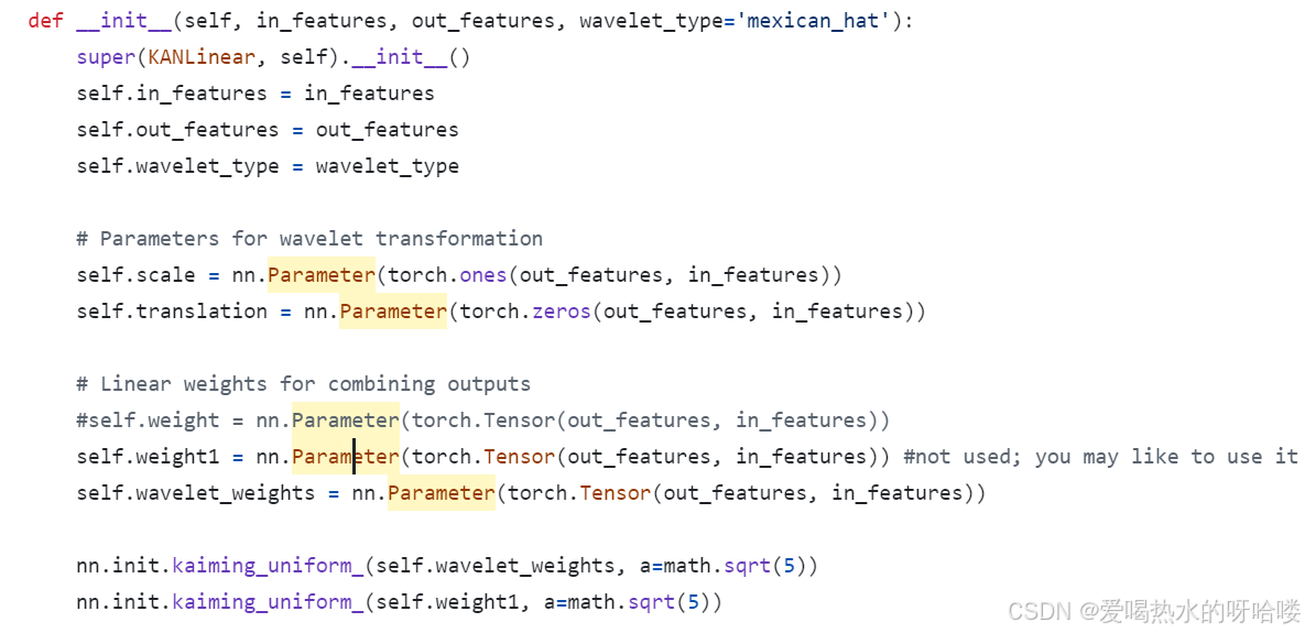
    def __init__(self, in_features, out_features, wavelet_type='mexican_hat'):
        super(KANLinear, self).__init__()
        self.in_features = in_features
        self.out_features = out_features
        self.wavelet_type = wavelet_type

        # Parameters for wavelet transformation
        self.scale = nn.Parameter(torch.ones(out_features, in_features))
        self.translation = nn.Parameter(torch.zeros(out_features, in_features))

        # Linear weights for combining outputs
        #self.weight = nn.Parameter(torch.Tensor(out_features, in_features))
        self.weight1 = nn.Parameter(torch.Tensor(out_features, in_features)) #not used; you may like to use it for wieghting base activation and adding it like Spl-KAN paper
        self.wavelet_weights = nn.Parameter(torch.Tensor(out_features, in_features))

        nn.init.kaiming_uniform_(self.wavelet_weights, a=math.sqrt(5))
        nn.init.kaiming_uniform_(self.weight1, a=math.sqrt(5))

        # Base activation function #not used for this experiment
        self.base_activation = nn.SiLU()

        # Batch normalization
        self.bn = nn.BatchNorm1d(out_features)

    def wavelet_transform(self, x):
        if x.dim() == 2:
            x_expanded = x.unsqueeze(1)
        else:
            x_expanded = x

        translation_expanded = self.translation.unsqueeze(0).expand(x.size(0), -1, -1)
        scale_expanded = self.scale.unsqueeze(0).expand(x.size(0), -1, -1)
        x_scaled = (x_expanded - translation_expanded) / scale_expanded

        # Implementation of different wavelet types
        if self.wavelet_type == 'mexican_hat':
            term1 = ((x_scaled ** 2)-1)
            term2 = torch.exp(-0.5 * x_scaled ** 2)
            wavelet = (2 / (math.sqrt(3) * math.pi**0.25)) * term1 * term2
            wavelet_weighted = wavelet * self.wavelet_weights.unsqueeze(0).expand_as(wavelet)
            wavelet_output = wavelet_weighted.sum(dim=2)
        elif self.wavelet_type == 'morlet':
            omega0 = 5.0  # Central frequency
            real = torch.cos(omega0 * x_scaled)
            envelope = torch.exp(-0.5 * x_scaled ** 2)
            wavelet = envelope * real
            wavelet_weighted = wavelet * self.wavelet_weights.unsqueeze(0).expand_as(wavelet)
            wavelet_output = wavelet_weighted.sum(dim=2)
            
        elif self.wavelet_type == 'dog':
            # Implementing Derivative of Gaussian Wavelet 
            dog = -x_scaled * torch.exp(-0.5 * x_scaled ** 2)
            wavelet = dog
            wavelet_weighted = wavelet * self.wavelet_weights.unsqueeze(0).expand_as(wavelet)
            wavelet_output = wavelet_weighted.sum(dim=2)
        elif self.wavelet_type == 'meyer':
            # Implement Meyer Wavelet here
            # Constants for the Meyer wavelet transition boundaries
            v = torch.abs(x_scaled)
            pi = math.pi

            def meyer_aux(v):
                return torch.where(v <= 1/2,torch.ones_like(v),torch.where(v >= 1,torch.zeros_like(v),torch.cos(pi / 2 * nu(2 * v - 1))))

            def nu(t):
                return t**4 * (35 - 84*t + 70*t**2 - 20*t**3)
            # Meyer wavelet calculation using the auxiliary function
            wavelet = torch.sin(pi * v) * meyer_aux(v)
            wavelet_weighted = wavelet * self.wavelet_weights.unsqueeze(0).expand_as(wavelet)
            wavelet_output = wavelet_weighted.sum(dim=2)
        elif self.wavelet_type == 'shannon':
            # Windowing the sinc function to limit its support
            pi = math.pi
            sinc = torch.sinc(x_scaled / pi)  # sinc(x) = sin(pi*x) / (pi*x)

            # Applying a Hamming window to limit the infinite support of the sinc function
            window = torch.hamming_window(x_scaled.size(-1), periodic=False, dtype=x_scaled.dtype, device=x_scaled.device)
            # Shannon wavelet is the product of the sinc function and the window
            wavelet = sinc * window
            wavelet_weighted = wavelet * self.wavelet_weights.unsqueeze(0).expand_as(wavelet)
            wavelet_output = wavelet_weighted.sum(dim=2)
            #You can try many more wavelet types ...
        else:
            raise ValueError("Unsupported wavelet type")

        return wavelet_output

    def forward(self, x):
        wavelet_output = self.wavelet_transform(x)
        #You may like test the cases like Spl-KAN
        #wav_output = F.linear(wavelet_output, self.weight)
        #base_output = F.linear(self.base_activation(x), self.weight1)

        base_output = F.linear(x, self.weight1)
        combined_output =  wavelet_output #+ base_output 

        # Apply batch normalization
        return self.bn(combined_output)

class KAN(nn.Module):
    def __init__(self, layers_hidden, wavelet_type='mexican_hat'):
        super(KAN, self).__init__()
        self.layers = nn.ModuleList()
        for in_features, out_features in zip(layers_hidden[:-1], layers_hidden[1:]):
            self.layers.append(KANLinear(in_features, out_features, wavelet_type))

    def forward(self, x):
        for layer in self.layers:
            x = layer(x)
        return x

这段代码定义了一个名为 KAN 的 PyTorch 模块，它实现了一个基于小波变换的神经网络，称为 Wavelet Kolmogorov-Arnold Networks (Wav-KAN)。以下是代码的详细解释：

类定义和初始化

class KANLinear(nn.Module):
    def __init__(self, in_features, out_features, wavelet_type='mexican_hat'):
        super(KANLinear, self).__init__()
        # ... 省略了一些初始化代码 ...

• KANLinear 类继承自 nn.Module，是一个自定义的神经网络层，它结合了小波变换和线性变换。
• in_features 和 out_features 分别是输入和输出特征的维度。
• wavelet_type 是一个字符串，指定了使用哪种类型的小波变换。

小波变换方法

def wavelet_transform(self, x):
    # ... 省略了小波变换的实现代码 ...

• wavelet_transform 方法实现了不同类型的小波变换，包括墨西哥帽（Mexican Hat）、莫莱（Morlet）、高斯导数（DOG）、梅耶（Meyer）和香农（Shannon）小波。
• 对于每种小波类型，该方法计算小波变换并加权求和。

参数在这里

可学习的参数（Learnable Parameters）：

• self.scale：一个 nn.Parameter，表示小波变换的缩放因子，它在训练过程中会被优化。
• self.translation：一个 nn.Parameter，表示小波变换的平移因子，它在训练过程中会被优化。
• self.wavelet_weights：一个 nn.Parameter，用于在小波变换后对结果进行加权，它在训练过程中会被优化。
• self.weight1：一个 nn.Parameter，虽然注释中提到这个参数在这个实验中没有使用，但它是一个可学习的权重参数，如果被使用，它也会在训练过程中被优化。

不可学习的参数（Non-Learnable Parameters）：

• self.in_features 和 self.out_features：这两个参数分别表示输入和输出特征的维度，它们是固定的，不会在训练过程中被优化。
• self.wavelet_type：这是一个字符串，指定了使用哪种类型的小波变换，它不是参数，而是一个配置选项，不会在训练过程中被优化。
• self.base_activation：这是一个 nn.SiLU() 激活函数，它是固定的，不会在训练过程中被优化。
• self.bn：这是一个批量归一化层，它包含可学习的参数（如权重和偏置），但是在这个上下文中，我们通常不将批量归一化层的参数单独列出，因为它们是批量归一化层内部的一部分。

在 PyTorch 中，nn.Parameter 是用来指定需要通过梯度下降进行优化的参数。其他的属性，如整数、浮点数或字符串，通常不被视为可学习的参数，因为它们在训练过程中保持不变。

关于小波变换的参数：放缩和平移

关于整合输出的参数：权重矩阵& 

前向传播方法

def forward(self, x):
    wavelet_output = self.wavelet_transform(x)
    # ... 省略了一些可能的代码路径 ...
    combined_output = wavelet_output  # + base_output 
    return self.bn(combined_output)

• forward 方法实现了前向传播，首先对小波变换的输出进行加权求和，然后通过批量归一化（Batch Normalization）。

KAN 类

class KAN(nn.Module):
    def __init__(self, layers_hidden, wavelet_type='mexican_hat'):
        super(KAN, self).__init__()
        self.layers = nn.ModuleList()
        for in_features, out_features in zip(layers_hidden[:-1], layers_hidden[1:]):
            self.layers.append(KANLinear(in_features, out_features, wavelet_type))

    def forward(self, x):
        for layer in self.layers:
            x = layer(x)
        return x

• KAN 类继承自 nn.Module，是一个完整的神经网络模型，由多个 KANLinear 层组成。
• layers_hidden 是一个列表，指定了每个隐藏层的输入和输出特征维度。
• 在 forward 方法中，输入 x 通过所有 KANLinear 层进行前向传播。

总结

这段代码定义了一个结合了小波变换和线性变换的神经网络模型。模型的核心是 KANLinear 层，它使用不同类型的小波变换来处理输入数据，然后通过线性变换和批量归一化来生成输出。KAN 类将这些层堆叠起来，形成一个深度神经网络。

一般性的

一个概念性的解释，假设这段代码是实现了一个类似的过程：

1. 小波变换层： 在神经网络中，小波函数可以用来作为层的一部分，类似于传统的激活函数。在小波变换层中，输入数据会通过一系列的小波函数进行变换。这些小波函数通常具有局部性和多尺度特性，这使得它们非常适合捕捉数据的局部特征。

2. 参数化的小波变换： 在代码中，self.scale 和 self.translation 是可学习的参数，它们用于调整小波函数的缩放和平移。这些参数使得小波函数能够根据输入数据的特点进行适配，从而更好地逼近目标函数。

3. 逼近过程：

   • 输入数据的前向传播：输入数据 x 通过神经网络的前向传播过程，在每个 KANLinear 层中，数据首先通过小波变换进行处理。
   • 小波变换：具体来说，输入数据与小波函数的缩放和平移版本进行卷积（或类似操作）。例如，如果使用墨西哥帽小波，那么每个神经元可能会计算如下公式：

     ​)

     其中，�a 是缩放因子，�b 是平移因子，�ψ 是小波函数。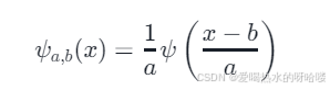
   • 加权：变换后的数据会与可学习权重 self.wavelet_weights 相乘，这进一步调整了小波变换的输出，使其更适合逼近目标函数。
   • 非线性激活：在某些情况下，小波变换的输出可能会通过一个非线性激活函数，如 SiLU，以引入非线性特性，这对于逼近复杂函数是必要的。

4. 训练过程： 在训练过程中，通过比较网络的输出和目标值，计算损失函数。然后，使用反向传播算法来调整网络中的可学习参数（包括小波函数的缩放和平移参数），以减少损失函数的值。这个过程迭代进行，直到网络输出与目标值足够接近，从而实现了函数逼近。

总结来说，这段代码中使用小波函数进行逼近的方法涉及将输入数据通过一系列参数化的小波变换层，然后通过反向传播算法优化这些参数，使得网络的输出能够逼近目标函数。由于具体的实现细节没有在代码中给出，这里的解释是基于一般的小波神经网络原理。