NetworkD3 | 让我们一起画个动态的桑基图吧~

1写在前面

桑基图（Sankey diagram），即桑基能量分流图，也叫桑基能量平衡图，应用场景非常广泛，举个栗子：ceRNA调控网络等。😉

本期我们画一个不一样的桑基图吧，可视实现动态交互。🤗

2用到的包

rm(list = ls())
library(tidyverse)
library(visNetwork)
library(networkD3)
library(igraph)

3示例数据

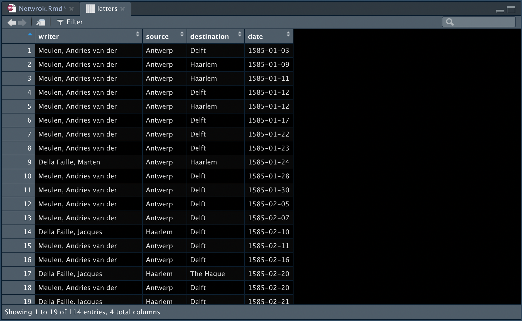
本次使用的示例数据是Daniel van der Meulen在1585年收到的信件所组成，包括writer,source, destination和date。 🥰

letters <- read.csv("correspondence-data-1585.csv")

4整理nodes数据

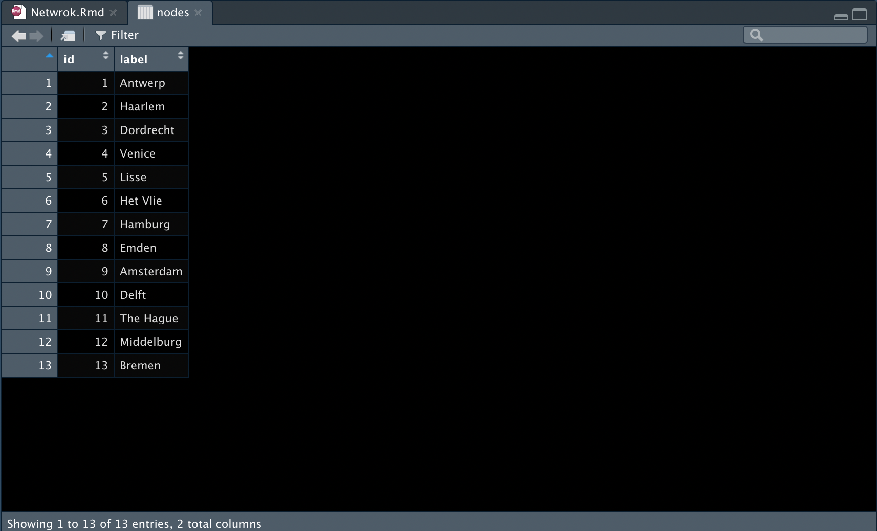
我们将source和destination提取出来并去重，整理为nodes文件；😘
同时，我们为每一个城市创建一个ID。😉

sources <- letters %>%
  distinct(source) %>%
  rename(label = source)

destinations <- letters %>%
  distinct(destination) %>%
  rename(label = destination)

nodes <- full_join(sources, destinations, by = "label")%>% 
  rowid_to_column("id")

5整理edges数据

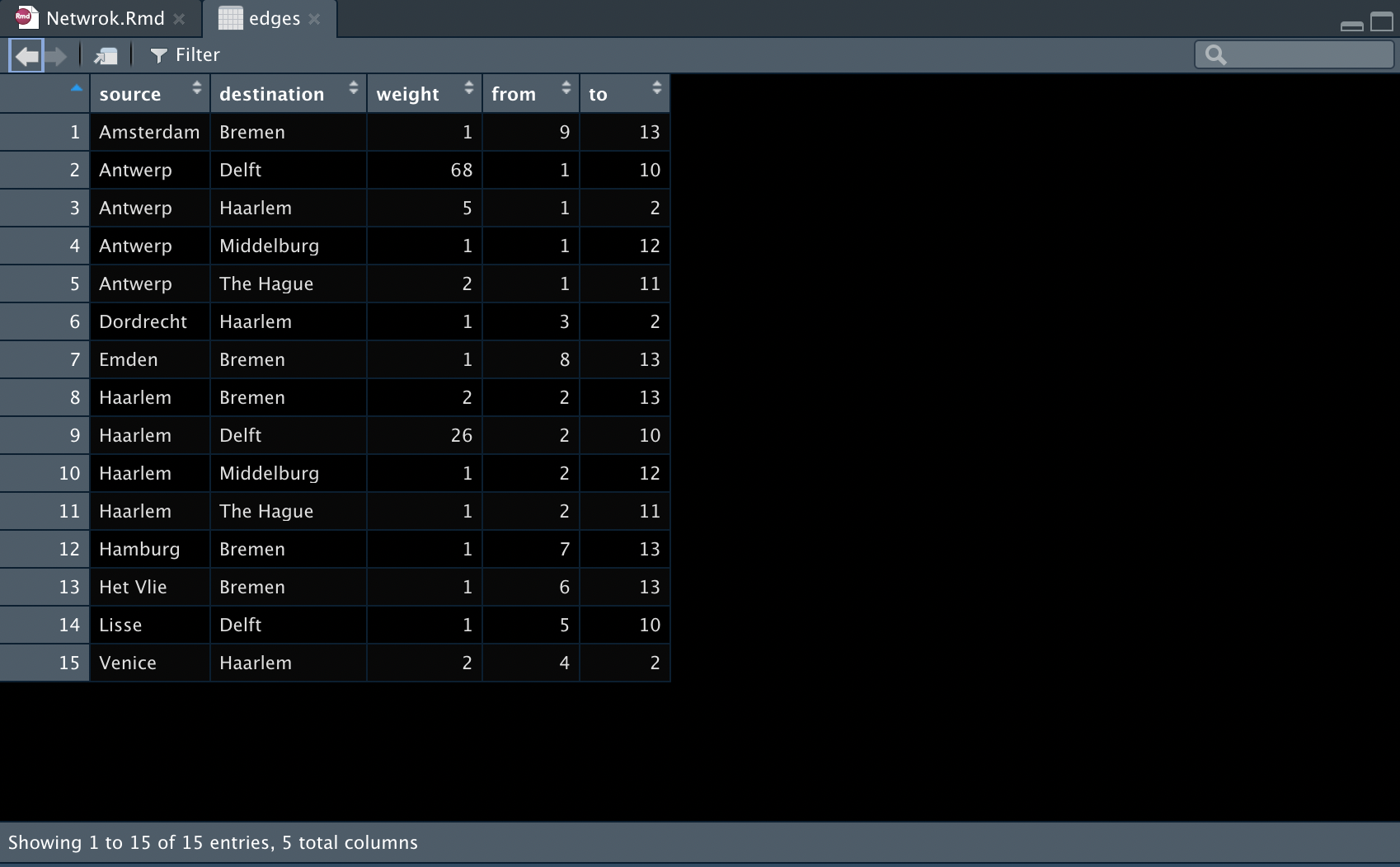
整理edges文件与nodes文件类似；🤒
在此，我们计算一下从source城市到destination城市间的来信次数，定义为weight；🥰
后面我们会以weight定义边的粗细；
最后我们将nodes文件中的ID加入。🤩

edges <- letters %>%  
  group_by(source, destination) %>% 
  summarise(weight = n()) %>% 
  ungroup() %>% 
  left_join(nodes, by = c("source" = "label")) %>% 
  rename(from = id) %>% 
  left_join(nodes, by = c("destination" = "label")) %>% 
  rename(to = id)

edges <- edges %>% 
  dplyr::select(., from, to, weight)

6进一步整理数据

Note! 这里需要注意的是，networkD3输入文件的ID需要从0开始计数。🫠
所以，这里我们需要重新更改一下ID。🌟

nodes_d3 <- mutate(nodes, id = id - 1)
edges_d3 <- mutate(edges, from = from - 1, to = to - 1)

7桑基图

sankeyNetwork(Links = edges_d3, Nodes = nodes_d3, Source = "from", Target = "to", 
              NodeID = "label", Value = "weight", fontSize = 16, unit = "Letter(s)")

---

最后祝大家早日不卷!~

---

需要示例数据的小伙伴，在公众号回复Sankey获取吧！

点个在看吧各位~ ✐.ɴɪᴄᴇ ᴅᴀʏ 〰

本文由 mdnice 多平台发布