


文章目录
- 1.库和数据导入
- 2.处理特征
- 2.1特征含义匹配
- 2.2目标值简单分析
- 2.2.1房价
- 2.2.2面积
- 2.2.3销售类型
- 2.2.4建筑类别、分区
- 2.2.5是否临街
- 2.2.6建筑面积
- 2.2.7 街道、胡同数目
- 2.2.8房屋大致形状
- 2.2.9物业
- 2.2.10公共设施可用度
- 2.2.11内部配置
- 2.2.12坡度
- 2.2.13周围位置
- 2.2.14住宅风格
- 2.2.15建筑材料和施工质量
- 2.2.16总体状况评级
- 2.2.17建造年份
- 2.2.18改造日期
- 2.2.19地基类型
- 2.2.20地下室高度
- 2.2.21Type 1地下室建筑面积
- 2.2.22BsmtCond地下室评分
- 2.2.23未完工地下室总面积、地下室总面积
- 2.2.24光照类型
- 2.2.25一楼面积
- 2.2.26二楼面积
- 2.2.27低质量建筑面积
- 2.2.28地上生活区面积
- 2.2.29齐全的高档洗浴间
- 2.2.30齐全的洗浴间
- 2.2.31高档房间数
- 2.2.32实用等级
- 2.2.33车库位置
- 2.2.33车库库龄
- 2.2.34车库的内部装饰
- 2.2.35车库存车量
- 2.2.36车库面积
- 2.2.37车库质量
- 2.2.38车库评分
- 2.2.39木阳台面积
- 2.2.40OpenPorchSF
- 2.2.41封闭门廊面积
- 2.2.42三季门廊面积
- 2.2.43屏风门廊面积
- 2.2.44泳池面积、质量
- 2.2.45杂余项
- 2.2.46墙体贴面类型
- 2.2.47墙体贴面的面积
- 2.2.48第二个建筑面积 (如果存在)
- 2.2.49杂余项2
- 2.3相关性分析
- 2.4标准化
- 3.建模与预测
1.库和数据导入
1.1库的导入
# 基础库导入
import pandas as pd
import numpy as np

# 可视化
import matplotlib.pyplot as plt
import seaborn as sns

# 高级计算库
from scipy import stats
from scipy.stats import  norm

# 机器学习库的导入
from sklearn.preprocessing import StandardScaler
from sklearn.impute import SimpleImputer
import sklearn
1.2 删除警告消息
#通过警告过滤器进行控制是否发出警告消息
import warnings
warnings.filterwarnings('ignore')
1.3导入csv数据
# 导入train训练集和test测试集
train = pd.read_csv(r'Desktop\train.csv',index_col = "Id")
test = pd.read_csv(r'Desktop\test.csv',index_col = "Id")
print(train.shape)
print(test.shape)
(1460, 80)
(1459, 79)
2.处理特征
步骤分析:
- 查看每个特征的构成
- 填补缺失
- 查看每个特征的分布
- 偏态正态化
- 构造新特征
- 删除不需要特征
- 删除异常值
2.1特征含义匹配
- 房价受诸多因素影响,本次比赛提供了房屋的很多信息以及最终房屋的价格。
- 我们需要用这些数据训练波形,最终来预测其他房屋的价格。
以下为本组的中文含义定义:
| 特征 | 含义 | 特征 | 含义 |
|---|---|---|---|
| SalePrice | 房价 | MSSubClass | 建筑的类别 |
| MSZoning | 分区(难道是穷人区和富人区?) | LotFrontage | 临街,越靠近街道价格越高 |
| LotArea | 面积 | Street | 街道 |
| Alley | 胡同 | LotShape | 房屋的大致形状 |
| LandContour | 物业 | Utilities | 公共设施可用度 |
| LotConfig | 配置 | LandSlope | 坡度 |
| Neighborhood | 位置 | Condition1 | 靠近铁路公路 |
| Condition2 | 靠近铁路公路(如果存在第二个) | BldgType | 住宅类型 |
| HouseStyle | 房屋风格 | OverallQual | 建筑材料和施工质量 |
| OverallCond | 总体状况评级 | YearBuilt | 建造年份 |
| YearRemodAdd | 改造日期 | RoofStyle | 屋顶类型 |
| RoofMatl | 屋顶材料 | Exterior1st | 外部覆盖物 |
| Exterior2nd | 外部覆盖物 (如果有第二种) | MasVnrType | 墙体贴面类型 |
| MasVnrArea | 墙体贴面的面积 | ExterQual | 贴面的质量 |
| ExterCond | 外部材料状况 | Foundation | 地基类型 |
| BsmtQual | 地下室高度 | BsmtCond | 地下室评分 |
| BsmtExposure | 花园层地下室墙壁 | BsmtFinType1 | 地下室施工质量 |
| BsmtFinSF1 | Type 1 建筑面积 | BsmtFinType2 | 第二个建筑面积 (如果存在) |
| BsmtFinSF2 | Type 2 建筑面积 | BsmtUnfSF | 未完成地下室面积 |
| TotalBsmtSF | 地下室总面积 | Heating | 光照类型 |
| HeatingQC | 光照质量与类型 | CentralAir | 中央空调 |
| Electrical | 电力系统(国外有别墅房顶是太阳能发电板的) | 1stFlrSF | 一楼面积 |
| 2ndFlrSF | 二楼面积 | LowQualFinSF | 低质量建筑面积 |
| GrLivArea | 地上生活区面积 | BsmtFullBath | 齐全的洗浴间 |
| BsmtHalfBath | 地下室有洗浴间 | FullBath | 齐全的高档洗浴间 |
| HalfBath | 地下室有高档洗浴间 | BedroomAbvGr | 地上卧室数 |
| KitchenAbvGr | 厨房数 | KitchenQual | 厨房质量 |
| TotRmsAbvGrd | 高档房间数 | Functional | 实用等级 |
| Fireplaces | 壁炉数量 | FireplaceQu | 壁炉质量 |
| GarageType | 车库位置 | GarageYrBlt | 车库库龄 |
| GarageFinish | 车库的内部装饰 | GarageCars | 车库存车量 |
| GarageArea | 车库面积 | GarageQual | 车库质量 |
| GarageCond | 车库评分 | PavedDrive | 车道 |
| WoodDeckSF | 木阳台面积 | OpenPorchSF | 开放门廊面积 |
| EnclosedPorch | 封闭门廊面积 | 3SsnPorch | 三季门廊面积 |
| ScreenPorch | 屏风门廊面积 | PoolArea | 泳池面积 |
| PoolQC | 泳池质量 | Fence | 围栏质量 |
| MiscFeature | 杂项功能 | MiscVal | 其他功能的价值 |
| MoSold | 已售月份 | YrSold | 已售年份 |
| SaleType | 出售类型 | SaleCondition | 销售状况 |
2.2目标值简单分析
2.2.1房价
# SalePrice  房价

train['SalePrice'].value_counts()# 计算拥有的值和相应频率
train['SalePrice'].isnull().sum()# 检查数据是否丢失
train['SalePrice'] = np.log1p(train['SalePrice'])# 由于房价是有偏度的,将房价对数化
sns.distplot(train['SalePrice'], fit=norm)# 显示直方图及核密度估计

# 绘制PP图,观察目标分布与理论正态分布的区别
fig = plt.figure()
res = stats.probplot(train['SalePrice'], plot=plt)


- 对目标列进行拟合正态分布,得到最接近真实数据的标准正态分布曲线。
- 使用PP图将理论的正态分布图和实际的分布图作对比,得出的目标值接近正态分布。
2.2.2面积
# totalArea 整体的面积(地上生活区 + 车库 + 地下室)

train['totalArea'] = train['GrLivArea'] + train['GarageArea'] + train['TotalBsmtSF']
train = train.drop(train[train['totalArea'] > 8000].index)
train['totalArea'] = np.log1p(train['totalArea'])

# 显示直方图及核密度估计
sns.distplot(train['totalArea'], fit=norm)
# 绘制PP图,观察目标分布与理论正态分布的区别
fig = plt.figure()
res = stats.probplot(train['totalArea'], plot=plt)
# 分析面积特征与价格的关系
fig = plt.figure()
plt.plot(train['totalArea'],train['SalePrice'],'o')

# test空值填充
test['GrLivArea'] = test['GrLivArea'].fillna(0)
test['GarageArea'] = test['GarageArea'].fillna(0)
test['TotalBsmtSF'] = test['TotalBsmtSF'].fillna(0)
test['totalArea'] = test['GrLivArea'] + test['GarageArea'] + test['TotalBsmtSF']
test['totalArea'] = np.log1p(test['totalArea'])


- 对目标列进行拟合正态分布,得到最接近真实数据的标准正态分布曲线。
- 使用PP图将理论的正态分布图和实际的分布图作对比,得出的目标值接近正态分布。
- 显然,面积与价格有很强的线性关系。
2.2.3销售类型
# SaleCondition 销售类型

# 去掉个别不相干的值
print(train['SaleCondition'].value_counts())
# train['SaleCondition'].isnull().sum()
train = train[train['SaleCondition'] == 'Normal']
train = train.drop(train[train['GrLivArea'] > 4000].index)

# 绘制散点图
plt.plot(train['GrLivArea'][train['SaleCondition'] == 'Normal'],train['SalePrice'][train['SaleCondition'] == 'Normal'],'o')
plt.plot(train['GrLivArea'][train['SaleCondition'] == 'Partial'],train['SalePrice'][train['SaleCondition'] == 'Partial'],'o')
plt.plot(train['GrLivArea'][train['SaleCondition'] == 'Abnorml'],train['SalePrice'][train['SaleCondition'] == 'Abnorml'],'o')
plt.plot(train['GrLivArea'][train['SaleCondition'] == 'Family'],train['SalePrice'][train['SaleCondition'] == 'Family'],'o')
plt.plot(train['GrLivArea'][train['SaleCondition'] == 'Alloca'],train['SalePrice'][train['SaleCondition'] == 'Alloca'],'o')
plt.plot(train['GrLivArea'][train['SaleCondition'] == 'AdjLand'],train['SalePrice'][train['SaleCondition'] == 'AdjLand'],'o')
Normal     1198
Partial     123
Abnorml     101
Family       20
Alloca       12
AdjLand       4
Name: SaleCondition, dtype: int64


[<matplotlib.lines.Line2D at 0x2939f8ae970>]

- 由散点图的趋势可获得显而易见的结果:面积与价格有很强的线性关系。
- 六种不同的销售条件的情况下,在销售条件相同时,考虑地上生活区面积与出售价格,得到二者成一定的线性关系。
2.2.4建筑类别、分区
# MSSubClass 建筑类别、分区

# 探究该特征的值的分布、去掉个别不相干的值
print(train['MSZoning'].value_counts())
train['SaleCondition'].isnull().sum()
train = train.drop(train[(train['GrLivArea'] > 3000) & (train['MSZoning'] == 'RM')].index)
train = train.drop(train[(train['GrLivArea'] > 3000) & (train['MSZoning'] == 'RH')].index)

# 绘制散点图
plt.plot(train['GrLivArea'][train['MSZoning'] == 'RL'],train['SalePrice'][train['MSZoning'] == 'RL'],'o')
plt.plot(train['GrLivArea'][train['MSZoning'] == 'RM'],train['SalePrice'][train['MSZoning'] == 'RM'],'o')
plt.plot(train['GrLivArea'][train['MSZoning'] == 'FV'],train['SalePrice'][train['MSZoning'] == 'FV'],'o')
plt.plot(train['GrLivArea'][train['MSZoning'] == 'RH'],train['SalePrice'][train['MSZoning'] == 'RH'],'o')
plt.plot(train['GrLivArea'][train['MSZoning'] == 'C (all)'],train['SalePrice'][train['MSZoning'] == 'C (all)'],'o')

#test集中用RL填充空值
test['MSZoning'] = test['MSZoning'].fillna('RL')
RL         954
RM         189
FV          39
RH          11
C (all)      4
Name: MSZoning, dtype: int64

- 由散点图的趋势可获得显而易见的结果:不同的房屋分区、类型,价格分布有明显不同,且结果具有显著性。
- 五种不同的建筑类型的情况下,在建筑类型相同时,考虑地上生活区面积与出售价格,得到二者成一定的线性关系。
2.2.5是否临街
# LotFrontage 临街

# 去掉个别不相干的值、填充完整此列
# print(train['LotFrontage'].value_counts().sort_index())
train = train.drop(train[train['LotFrontage'] > 300].index)
train['LotFrontage'] = train['LotFrontage'].fillna(train['LotFrontage'].mean())
train['not_LotFrontage'] = pd.Series(np.zeros((len(train))),index = train.index)
train['not_LotFrontage'][train['LotFrontage'] < 25] = 1
index = train['LotFrontage'] > 25

# 对数化处理、绘图
train['LotFrontage'] = np.log1p(train['LotFrontage'])
# train['LotFrontage'].isnull().sum()
sns.distplot(train['LotFrontage'], fit=norm)
fig = plt.figure()
res = stats.probplot(train['LotFrontage'][index], plot=plt)

# test集整理数据
test['LotFrontage'] = test['LotFrontage'].fillna(test['LotFrontage'].mean())
test['not_LotFrontage'] = pd.Series(np.zeros((len(test))),index = test.index)
test['not_LotFrontage'][test['LotFrontage'] < 25] = 1
test['LotFrontage'] = np.log1p(test['LotFrontage'])


- 由图易得在对数化处理后,拟合效果不能很好匹配。
- 使用PP图得出的目标值在小于-1和大于2时,偏离正态分布趋势。
2.2.6建筑面积
# LotArea建筑面积

# 去掉个别不相干的值
# print(train['LotArea'].value_counts().sort_index())
train = train.drop(train[train['LotArea'] > 100000].index)

# 对数化处理、绘图
train['LotArea'] = np.log1p(train['LotArea'])
sns.distplot(train['LotArea'], fit=norm)
fig = plt.figure()
res = stats.probplot(train['LotArea'], plot=plt)
fig = plt.figure()
plt.plot(train['LotArea'],train['SalePrice'],'o')

# test对数化处理
test['LotArea'] = np.log1p(test['LotArea'])


- 由图易得在对数化处理后,拟合效果不能很好匹配。
- 使用PP图得出的目标值在小于-1和大于2时,偏离正态分布趋势。
- 由散点图的趋势可得:面积与价格有不具备显著的线性关系。
2.2.7 街道、胡同数目
# Street Alley 街道 胡同

# 探究两个特征的值的分布
print(train['Street'].value_counts().sort_index())
print(train['Alley'].value_counts().sort_index())

# 数据量过少,可排除处理
train = train.drop('Street', axis=1)
train = train.drop('Alley', axis=1)
test = test.drop('Street', axis=1)
test = test.drop('Alley', axis=1)
Grvl       4
Pave    1186
Name: Street, dtype: int64
Grvl    43
Pave    28
Name: Alley, dtype: int64
*数据量过少,可排除处理
2.2.8房屋大致形状
# LotShape 房屋大致形状

# 探究该特征的值的分布
print(train['LotShape'].value_counts().sort_index())
print(train['LotShape'].isnull().sum()/len(train))

# 绘制散点图
plt.plot(train['GrLivArea'][train['LotShape'] == 'IR1'],train['SalePrice'][train['LotShape'] == 'IR1'],'o')
plt.plot(train['GrLivArea'][train['LotShape'] == 'Reg'],train['SalePrice'][train['LotShape'] == 'Reg'],'o')
plt.plot(train['GrLivArea'][train['LotShape'] == 'IR2'],train['SalePrice'][train['LotShape'] == 'IR2'],'o')
plt.plot(train['GrLivArea'][train['LotShape'] == 'IR3'],train['SalePrice'][train['LotShape'] == 'IR3'],'o')
IR1    396
IR2     31
IR3      6
Reg    757
Name: LotShape, dtype: int64
0.0


[<matplotlib.lines.Line2D at 0x2939f9a7610>]

- 由散点图的趋势可获得显而易见的结果:不同的房屋形状最终价格分布均在一定范围内,不具有显著性。
- 四种不同的房屋形状的情况下,在房屋形状相同时,考虑地上生活区面积与出售价格,得到二者成一定的线性关系。
2.2.9物业
# LandContour 物业

# 探究该特征的值的分布
print(train['LandContour'].value_counts().sort_index())
print(train['LandContour'].isnull().sum()/len(train))

# 绘制散点图
plt.plot(train['GrLivArea'][train['LandContour'] == 'Lvl'],train['SalePrice'][train['LandContour'] == 'Lvl'],'o')
plt.plot(train['GrLivArea'][train['LandContour'] == 'Bnk'],train['SalePrice'][train['LandContour'] == 'Bnk'],'o')
plt.plot(train['GrLivArea'][train['LandContour'] == 'HLS'],train['SalePrice'][train['LandContour'] == 'HLS'],'o')
plt.plot(train['GrLivArea'][train['LandContour'] == 'Low'],train['SalePrice'][train['LandContour'] == 'Low'],'o')
Bnk      49
HLS      33
Low      29
Lvl    1079
Name: LandContour, dtype: int64
0.0


[<matplotlib.lines.Line2D at 0x293a09d1f70>]

- 由散点图的趋势可获得显而易见的结果:不同的物业情况下,最终价格分布均在一定范围内,不具有显著性。
- 四种不同的物业的情况下,在物业选择相同时,考虑地上生活区面积与出售价格,得到二者不成一定的线性关系。
2.2.10公共设施可用度
# Utilities 公共设施可用度

# 探究该特征的值的分布
print(train['Utilities'].value_counts().sort_index())
print(train['Utilities'].isnull().sum()/len(train))

# 数据量过少,可排除处理
train = train.drop('Utilities', axis=1)
test = test.drop('Utilities', axis=1)
AllPub    1190
Name: Utilities, dtype: int64
0.0
*数据量过少,可排除处理
2.2.11内部配置
# LotConfig内部配置

# 探究该特征的值的分布
print(train['LotConfig'].value_counts().sort_index())
print(train['LotConfig'].isnull().sum()/len(train))

# 绘制散点图
plt.plot(train['GrLivArea'][train['LotConfig'] == 'Corner'],train['SalePrice'][train['LotConfig'] == 'Corner'],'o')
plt.plot(train['GrLivArea'][train['LotConfig'] == 'Inside'],train['SalePrice'][train['LotConfig'] == 'Inside'],'o')
plt.plot(train['GrLivArea'][train['LotConfig'] == 'CulDSac'],train['SalePrice'][train['LotConfig'] == 'CulDSac'],'o')
plt.plot(train['GrLivArea'][train['LotConfig'] == 'FR3'],train['SalePrice'][train['LotConfig'] == 'FR3'],'o')
Corner     209
CulDSac     77
FR2         42
FR3          4
Inside     858
Name: LotConfig, dtype: int64
0.0


[<matplotlib.lines.Line2D at 0x293a0a39910>]

- 由散点图的趋势可获得显而易见的结果:不同的内部配置情况下,最终价格分布均在一定范围内,不具有显著性。
- 四种不同的内部配置的情况下,在内部配置相同时,考虑地上生活区面积与出售价格,得到二者成一定的线性关系。
2.2.12坡度
# LandSlope 坡度

# 探究该特征的值的分布
print(train['LandSlope'].value_counts().sort_index())
print(train['LandSlope'].isnull().sum()/len(train))

# 绘制散点图
plt.plot(train['GrLivArea'][train['LandSlope'] == 'Gtl'],train['SalePrice'][train['LandSlope'] == 'Gtl'],'o')
plt.plot(train['GrLivArea'][train['LandSlope'] == 'Mod'],train['SalePrice'][train['LandSlope'] == 'Mod'],'o')
plt.plot(train['GrLivArea'][train['LandSlope'] == 'Sev'],train['SalePrice'][train['LandSlope'] == 'Sev'],'o')
Gtl    1130
Mod      55
Sev       5
Name: LandSlope, dtype: int64
0.0


[<matplotlib.lines.Line2D at 0x293a0a96880>]

- 由散点图的趋势可获得显而易见的结果:不同的坡度情况下,最终价格分布均在一定范围内,不具有显著性。
- 三种不同的坡度的情况下,在坡度相同时,考虑地上生活区面积与出售价格,得到二者成一定的线性关系。
2.2.13周围位置
# Neighborhood Condition1 Condition2位置

# 探究该特征的值的分布
print(train['Neighborhood'].value_counts().sort_index())
print(train['Neighborhood'].isnull().sum()/len(train))

print(train['Condition1'].value_counts().sort_index())
print(train['Condition1'].isnull().sum()/len(train))

print(train['Condition2'].value_counts().sort_index())
print(train['Condition2'].isnull().sum()/len(train))

# 绘制散点图
plt.plot(train['GrLivArea'][train['Condition1'] == 'Norm'],train['SalePrice'][train['Condition1'] == 'Norm'],'o')
plt.plot(train['GrLivArea'][train['Condition1'] == 'Artery'],train['SalePrice'][train['Condition1'] == 'Artery'],'o')
plt.plot(train['GrLivArea'][train['Condition1'] == 'Feedr'],train['SalePrice'][train['Condition1'] == 'Feedr'],'o')
Blmngtn     12
Blueste      2
BrDale      12
BrkSide     54
ClearCr     22
CollgCr    129
Crawfor     43
Edwards     82
Gilbert     64
IDOTRR      29
MeadowV     16
Mitchel     42
NAmes      197
NPkVill      8
NWAmes      64
NoRidge     36
NridgHt     45
OldTown     92
SWISU       22
Sawyer      67
SawyerW     50
Somerst     49
StoneBr     16
Timber      26
Veenker     11
Name: Neighborhood, dtype: int64
0.0
Artery      39
Feedr       67
Norm      1025
PosA         7
PosN        17
RRAe         8
RRAn        21
RRNe         2
RRNn         4
Name: Condition1, dtype: int64
0.0
Artery       1
Feedr        5
Norm      1179
PosA         1
RRAe         1
RRAn         1
RRNn         2
Name: Condition2, dtype: int64
0.0


[<matplotlib.lines.Line2D at 0x293a0afb970>]

- Neighborhood的数据值极度分散,不需要具体考虑。
- Condition2数据显著集中在‘Norm’值中,不需要具体考虑。
- 由散点图的趋势可获得显而易见的结果:不同的condition1,价格分布有明显不同,且结果具有显著性。
- 三种不同的建筑类型的情况下,在condition1相同时,考虑地上生活区面积与出售价格,得到二者成一定的线性关系。
2.2.14住宅风格
# BldgType住宅风格

# 探究该特征的值的分布
print(train['BldgType'].value_counts().sort_index())
print(train['BldgType'].isnull().sum()/len(train))

# 绘制散点图
plt.plot(train['GrLivArea'][train['BldgType'] == '1Fam'],train['SalePrice'][train['BldgType'] == '1Fam'],'o')
plt.plot(train['GrLivArea'][train['BldgType'] == '2fmCon'],train['SalePrice'][train['BldgType'] == '2fmCon'],'o')
plt.plot(train['GrLivArea'][train['BldgType'] == 'Duplex'],train['SalePrice'][train['BldgType'] == 'Duplex'],'o')
plt.plot(train['GrLivArea'][train['BldgType'] == 'TwnhsE'],train['SalePrice'][train['BldgType'] == 'TwnhsE'],'o')
plt.plot(train['GrLivArea'][train['BldgType'] == 'Twnhs'],train['SalePrice'][train['BldgType'] == 'Twnhs'],'o')
1Fam      999
2fmCon     27
Duplex     37
Twnhs      37
TwnhsE     90
Name: BldgType, dtype: int64
0.0


[<matplotlib.lines.Line2D at 0x293a0b60880>]

- 由散点图的趋势可获得显而易见的结果:不同的住宅风格情况下,最终价格分布均在一定范围内,不具有显著性。
- 五种不同的住宅风格的情况下,在住宅风格相同时,考虑地上生活区面积与出售价格,得到二者成一定的线性关系。
2.2.15建筑材料和施工质量
# OverallQual 建筑材料和施工质量

# 探究该特征的值的分布
print(train['OverallQual'].value_counts().sort_index())
print(train['OverallQual'].isnull().sum()/len(train))

# 对数化处理、绘图
sns.distplot(train['OverallQual'], fit=norm)
fig = plt.figure()
res = stats.probplot(train['OverallQual'], plot=plt)
fig = plt.figure()
plt.plot(train['OverallQual'],train['SalePrice'],'o')
1       2
2       2
3      16
4      98
5     340
6     327
7     252
8     120
9      25
10      8
Name: OverallQual, dtype: int64
0.0


[<matplotlib.lines.Line2D at 0x293a0c7aa90>]


- 对目标列进行拟合正态分布,得到最接近真实数据的标准正态分布曲线。
- 使用PP图将理论的正态分布图和实际的分布图作对比,得出的目标值接近正态分布。
- 显然,建筑材料和施工质量与价格有很强的线性关系。
2.2.16总体状况评级
# OverallCond 总体状况评级

# 探究该特征的值的分布、去掉个别不相干的值
print(train['OverallCond'].value_counts().sort_index())
print(train['OverallCond'].isnull().sum()/len(train))
train = train.drop(train[(train['OverallCond'] ==2 )&(train['SalePrice'] > 300000 )].index)

# 对数化处理、绘图
sns.distplot(train['OverallCond'], fit=norm)
fig = plt.figure()
res = stats.probplot(train['OverallCond'], plot=plt)
fig = plt.figure()
plt.plot(train['OverallCond'],train['SalePrice'],'o')
1      1
2      2
3     18
4     49
5    626
6    225
7    180
8     70
9     19
Name: OverallCond, dtype: int64
0.0


[<matplotlib.lines.Line2D at 0x2939f5f8c70>]


- 由图易得在对数化处理后,拟合效果不能很好匹配。
- 使用PP图得出的目标值在小于-2和大于1时,偏离正态分布趋势。
- 由散点图的趋势可得:面积与价格有不具备显著的线性关系。
2.2.17建造年份
# YearBuilt 建造年份

# 探究该特征的值的分布、去掉个别不相干的值
train['newhouse']  = pd.Series(np.zeros((len(train))),index = train.index)
train['newhouse'][train['YearBuilt'] > 2000]  = 1
train['age']  = 2010 - train['YearBuilt']
print(train['age'].value_counts().sort_index())
print(train['YearBuilt'].value_counts().sort_index())
print(train['YearBuilt'].isnull().sum()/len(train))

# 绘制散点图
plt.plot(train['YearBuilt'],train['SalePrice'],'o')

# test对数化处理
test['newhouse']  = pd.Series(np.zeros((len(test))),index = test.index)
test['newhouse'][test['YearBuilt'] > 2000]  = 1
test['age']  = 2010 - test['YearBuilt']
1       3
2       9
3      19
4      24
5      39
       ..
125     2
128     1
130     2
135     1
138     1
Name: age, Length: 110, dtype: int64
1872     1
1875     1
1880     2
1882     1
1885     2
        ..
2005    39
2006    24
2007    19
2008     9
2009     3
Name: YearBuilt, Length: 110, dtype: int64
0.0

- 由散点图的趋势可获得显而易见的结果:不同的建造年份,价格分布有明显不同,且结果具有显著性。
- 建造年份与出售价格,二者成一定的线性关系。
2.2.18改造日期
# YearRemodAdd 改造日期

# 探究该特征的值的分布、去掉个别不相干的值
print(train['YearRemodAdd'].value_counts().sort_index())
print(train['YearRemodAdd'].isnull().sum()/len(train))
train['1950house']  = pd.Series(np.zeros((len(train))),index = train.index)
train['1950house'][train['YearRemodAdd'] == 1950]  = 1

# 绘制散点图
sns.distplot(train['YearRemodAdd'], fit=norm)
fig = plt.figure()
res = stats.probplot(train['YearRemodAdd'], plot=plt)
fig = plt.figure()
plt.plot(train['YearRemodAdd'],train['SalePrice'],'o')

# test对数化处理
test['1950house']  = pd.Series(np.zeros((len(test))),index = test.index)
test['1950house'][test['YearRemodAdd'] == 1950]  = 1
1950    150
1951      3
1952      4
1953      8
1954     12
       ...
2006     48
2007     36
2008     22
2009      6
2010      1
Name: YearRemodAdd, Length: 61, dtype: int64
0.0


- 对目标列进行拟合正态分布,得到最接近真实数据的标准正态分布曲线。
- 使用PP图将理论的正态分布图和实际的分布图作对比,得出的目标值接近正态分布。
- 显然,改造日期与价格有很强的线性关系
2.2.19地基类型
# Foundation 地基类型

# 探究该特征的值的分布
print(train['Foundation'].value_counts().sort_index())
print(train['Foundation'].isnull().sum()/len(train))

# 绘制散点图
plt.plot(train['GrLivArea'][train['Foundation'] == 'BrkTil'],train['SalePrice'][train['Foundation'] == 'BrkTil'],'o')
plt.plot(train['GrLivArea'][train['Foundation'] == 'CBlock'],train['SalePrice'][train['Foundation'] == 'CBlock'],'o')
plt.plot(train['GrLivArea'][train['Foundation'] == 'PConc'],train['SalePrice'][train['Foundation'] == 'PConc'],'o')
BrkTil    124
CBlock    551
PConc     486
Slab       21
Stone       5
Wood        3
Name: Foundation, dtype: int64
0.0


[<matplotlib.lines.Line2D at 0x293a0ca11c0>]

- 由散点图的趋势可获得显而易见的结果:不同的地基类型情况下,最终价格分布均在一定范围内,不具有显著性。
- 三种不同的地基类型的情况下,在地基类型相同时,考虑地上生活区面积与出售价格,得到二者成一定的线性关系。
2.2.20地下室高度
# BsmtQual 地下室高度

# 填充空缺数据
train['BsmtQual'] = train['BsmtQual'].fillna("unknown")
train['BsmtCond'] = train['BsmtCond'].fillna("TA")
train['BsmtExposure'] = train['BsmtExposure'].fillna("unknown")
train['BsmtFinType1'] = train['BsmtFinType1'].fillna("unknown")

test['BsmtQual'] = test['BsmtQual'].fillna("unknown")
test['BsmtCond'] = test['BsmtCond'].fillna("TA")
test['BsmtExposure'] = test['BsmtExposure'].fillna("unknown")
test['BsmtFinType1'] = test['BsmtFinType1'].fillna("unknown")
*数据残缺不具备普遍意义。
2.2.21Type 1地下室建筑面积
# BsmtFinSF1 Type 1地下室建筑面积

# 探究该特征的值的分布
print(train['BsmtFinSF1'].value_counts())
print(train['BsmtFinSF1'].isnull().sum()/len(train))
train['noSF1']  = pd.Series(np.zeros((len(train))),index = train.index)
train['noSF1'][train['BsmtFinSF1'] == 0]  = 1

# 绘制散点图
plt.plot(train['BsmtFinSF1'],train['SalePrice'],'o')

# 填充test空缺值
test['BsmtFinSF1'] = test['BsmtFinSF1'].fillna(0)
test['BsmtFinSF2'] = test['BsmtFinSF2'].fillna(0)
test['noSF1']  = pd.Series(np.zeros((len(test))),index = test.index)
test['noSF1'][test['BsmtFinSF1'] == 0]  = 1
0      353
24       9
16       8
662      5
686      5
      ...
762      1
763      1
769      1
772      1
609      1
Name: BsmtFinSF1, Length: 554, dtype: int64
0.0

- 由散点图的趋势可获得显而易见的结果:不同的Type 1地下室建筑面积,价格分布有明显不同,且结果具有显著性。
- Type 1地下室建筑面积与出售价格,二者成一定的线性关系。
2.2.22BsmtCond地下室评分
# BsmtCond地下室评分

# 填充空缺数据
train['BsmtCond'] = train['BsmtCond'].fillna(0)
test['BsmtCond'] = test['BsmtCond'].fillna(0)
*数据残缺不具备普遍意义。
2.2.23未完工地下室总面积、地下室总面积
# BsmtUnfS、TotalBsmtSF、noTotalBsmtSF

# 探究该特征的值的分布、去掉个别不相干的值
print(train['BsmtUnfSF'].value_counts())
print(train['TotalBsmtSF'].isnull().sum()/len(train))
train['noTotalBsmtSF']  = pd.Series(np.zeros((len(train))),index = train.index)
train['noTotalBsmtSF'][train['TotalBsmtSF'] == 0]  = 1
index = train['TotalBsmtSF'] > 0

# 对数化处理、绘图
train['TotalBsmtSF'] = np.log1p(train['TotalBsmtSF'])
sns.distplot(train['TotalBsmtSF'][index], fit=norm)
fig = plt.figure()
res = stats.probplot(train['TotalBsmtSF'][index], plot=plt)
fig = plt.figure()
plt.plot(train['TotalBsmtSF'][index],train['SalePrice'][index],'o')

# 填充test空缺值、对数化
test['TotalBsmtSF'] = test['TotalBsmtSF'].fillna(0)
test['noTotalBsmtSF']  = pd.Series(np.zeros((len(test))),index = test.index)
test['noTotalBsmtSF'][test['TotalBsmtSF'] == 0]  = 1
test['TotalBsmtSF'] = np.log1p(test['TotalBsmtSF'])
0      100
384      8
572      7
300      6
319      5
      ...
778      1
779      1
783      1
784      1
568      1
Name: BsmtUnfSF, Length: 668, dtype: int64
0.0


- 由图易得在对数化处理后,拟合效果能很好匹配。
- 使用PP图得出的目标值在小于-2时,偏离正态分布趋势。
- 由散点图的趋势可得:面积与价格有不具备显著的线性关系。
2.2.24光照类型
# Heating 光照类型

# 填充空缺数据
train['Electrical'] = train['Electrical'].fillna('SBrkr')
test['Electrical'] = test['Electrical'].fillna('SBrkr')
*数据残缺不具备普遍意义。
2.2.25一楼面积
# 1stFlrSF 一楼面积

# 探究该特征的值的分布
print(train['1stFlrSF'].value_counts())
print(train['1stFlrSF'].isnull().sum()/len(train))

# 对数化处理、绘图
train['1stFlrSF'] = np.log1p(train['1stFlrSF'])
sns.distplot(train['1stFlrSF'], fit=norm)
fig = plt.figure()
res = stats.probplot(train['1stFlrSF'], plot=plt)
fig = plt.figure()
plt.plot(train['1stFlrSF'][index],train['SalePrice'][index],'o')

# test对数化处理
test['1stFlrSF'] = np.log1p(test['1stFlrSF'])
864     22
1040    15
912     12
848     11
894     10
        ..
1304     1
1307     1
1309     1
1310     1
2053     1
Name: 1stFlrSF, Length: 647, dtype: int64
0.0


- 由图易得在对数化处理后,拟合效果能较好匹配。
- 使用PP图得出的目标值在接近-3时,偏离正态分布趋势。
- 由散点图的趋势可得:面积与价格有不具备显著的线性关系。
2.2.26二楼面积
# 2ndFlrSF二楼面积

# 探究该特征的值的分布、针对个别值定义
print(train['2ndFlrSF'].value_counts())
print(train['2ndFlrSF'].isnull().sum()/len(train))
train['no2ndFlrSF']  = pd.Series(np.zeros((len(train))),index = train.index)
train['no2ndFlrSF'][train['2ndFlrSF'] == 0]  = 1

# 绘图图
sns.distplot(train['2ndFlrSF'], fit=norm)

# test数据定义、对数化处理
test['no2ndFlrSF']  = pd.Series(np.zeros((len(test))),index = test.index)
test['no2ndFlrSF'][test['2ndFlrSF'] == 0]  = 1
0       662
504       8
600       6
896       6
672       6
       ...
1243      1
838       1
836       1
834       1
1796      1
Name: 2ndFlrSF, Length: 358, dtype: int64
0.0

- 由图易得在对数化处理后,拟合效果不能很好匹配。
2.2.27低质量建筑面积
# LowQualFinSF 低质量建筑面积

# 探究该特征的值的分布、针对个别值定义
print(train['LowQualFinSF'].value_counts())
print(train['LowQualFinSF'].isnull().sum()/len(train))
train['haveLowQual']  = pd.Series(np.zeros((len(train))),index = train.index)
train['haveLowQual'][train['LowQualFinSF'] > 0]  = 1

# test数据定义
test['haveLowQual']  = pd.Series(np.zeros((len(test))),index = test.index)
test['haveLowQual'][test['LowQualFinSF'] > 0]  = 1
0      1170
80        2
360       2
479       1
473       1
420       1
397       1
390       1
384       1
514       1
234       1
232       1
205       1
156       1
144       1
120       1
481       1
53        1
528       1
Name: LowQualFinSF, dtype: int64
0.0
*数据极度集中,不具备普遍意义。
2.2.28地上生活区面积
# GrLivArea 地上生活区面积

# 探究该特征的值的分布
print(train['LowQualFinSF'].value_counts())
print(train['LowQualFinSF'].isnull().sum()/len(train))

# 对数化处理、绘图
train['GrLivArea'] = np.log1p(train['GrLivArea'])
sns.distplot(train['GrLivArea'], fit=norm);
fig = plt.figure()
res = stats.probplot(train['GrLivArea'], plot=plt)
fig = plt.figure()
plt.plot(train['GrLivArea'][index],train['SalePrice'][index],'o')

# test对数化处理
test['GrLivArea'] = np.log1p(test['GrLivArea'])
0      1170
80        2
360       2
479       1
473       1
420       1
397       1
390       1
384       1
514       1
234       1
232       1
205       1
156       1
144       1
120       1
481       1
53        1
528       1
Name: LowQualFinSF, dtype: int64
0.0


- 对目标列进行拟合正态分布,得到最接近真实数据的标准正态分布曲线。
- 使用PP图将理论的正态分布图和实际的分布图作对比,得出的目标值接近正态分布。
- 显然,地上生活区面积与价格有很强的线性关系。
2.2.29齐全的高档洗浴间
# FullBath 齐全的高档洗浴间

# 探究该特征的值的分布
print(train['FullBath'].value_counts())
print(train['FullBath'].isnull().sum()/len(train))

# 对数化处理、绘图
sns.distplot(train['FullBath'], fit=norm);
fig = plt.figure()
res = stats.probplot(train['FullBath'], plot=plt)
fig = plt.figure()
plt.plot(train['FullBath'],train['SalePrice'],'o')
2    606
1    563
3     16
0      5
Name: FullBath, dtype: int64
0.0


[<matplotlib.lines.Line2D at 0x293a0bca5e0>]


- 对目标列进行拟合正态分布,得到最接近真实数据的标准正态分布曲线。
- 使用PP图将理论的正态分布图和实际的分布图作对比,得出的目标值接近正态分布。
- 显然,齐全的高档洗浴间与价格有很强的线性关系。
2.2.30齐全的洗浴间
# BsmtFullBath 齐全的洗浴间

# 探究该特征的值的分布
print(train['BsmtFullBath'].value_counts())
print(train['BsmtFullBath'].isnull().sum()/len(train))

# 对数化处理、绘图
train['BsmtFullBath'] = np.log1p(train['BsmtFullBath'])
sns.distplot(train['BsmtFullBath'], fit=norm);
fig = plt.figure()
res = stats.probplot(train['BsmtFullBath'], plot=plt)
fig = plt.figure()
plt.plot(train['BsmtFullBath'],train['SalePrice'],'o')

# test对数化处理、部分的平均定义
test['BsmtFullBath'] = test['BsmtFullBath'].fillna(test['BsmtFullBath'].mean())
test['BsmtFullBath'] = np.log1p(test['BsmtFullBath'])
0    687
1    497
2      6
Name: BsmtFullBath, dtype: int64
0.0


- 由图易得在对数化处理后,拟合效果不能很好匹配。
- 使用PP图得出的目标值偏离正态分布趋势。
- 由散点图的趋势可得:齐全洗浴间的数目与价格有不具备显著的线性关系。
2.2.31高档房间数
# TotRmsAbvGrd高档房间数

# 探究该特征的值的分布
print(train['TotRmsAbvGrd'].value_counts())
print(train['TotRmsAbvGrd'].isnull().sum()/len(train))

# 对数化处理、绘图
train['TotRmsAbvGrd'] = np.log1p(train['TotRmsAbvGrd'])
sns.distplot(train['TotRmsAbvGrd'], fit=norm);
fig = plt.figure()
res = stats.probplot(train['TotRmsAbvGrd'], plot=plt)
fig = plt.figure()
plt.plot(train['TotRmsAbvGrd'],train['SalePrice'],'o')

# test对数化处理、部分的平均定义
test['TotRmsAbvGrd'] = test['TotRmsAbvGrd'].fillna(test['TotRmsAbvGrd'].mean())
test['TotRmsAbvGrd'] = np.log1p(test['TotRmsAbvGrd'])
6     328
7     267
5     243
8     150
4      77
9      58
10     33
3      16
11     10
12      7
2       1
Name: TotRmsAbvGrd, dtype: int64
0.0


- 对目标列进行拟合正态分布,得到最接近真实数据的标准正态分布曲线。
- 使用PP图将理论的正态分布图和实际的分布图作对比,得出的目标值接近正态分布。
- 显然,高档房间数与价格有很强的线性关系。
2.2.32实用等级
# Functional 实用等级

# 探究该特征的值的分布
print(train['Fireplaces'].value_counts())
print(train['Fireplaces'].isnull().sum()/len(train))

# 数据量过少,可排除处理
train = train.drop('FireplaceQu',axis=1)
test = test.drop('FireplaceQu',axis=1)
0    563
1    531
2     92
3      4
Name: Fireplaces, dtype: int64
0.0
*数据量过少,可排除处理
2.2.33车库位置
# GarageType 车库位置

# 探究该特征的值的分布
print(train['GarageType'].value_counts())
print(train['GarageType'].isnull().sum()/len(train))

# 填充空缺数据
train['GarageType'] = train['GarageType'].fillna('unknown')
test['GarageType'] = test['GarageType'].fillna('unknown')
Attchd     705
Detchd     337
BuiltIn     65
Basment     12
CarPort      6
2Types       4
Name: GarageType, dtype: int64
0.05126050420168067
*数据残缺不具备普遍意义。
2.2.33车库库龄
# GarageYrBlt 车库库龄

# 探究该特征的值的分布
print(train['GarageYrBlt'].value_counts())
print(train['GarageYrBlt'].isnull().sum()/len(train))

# 部分数据的平均定义
train['GarageYrBlt'] = train['GarageYrBlt'].fillna(train['GarageYrBlt'].mean())
test['GarageYrBlt'] = test['GarageYrBlt'].fillna(test['GarageYrBlt'].mean())

# 绘制散点图
plt.plot(train['GarageYrBlt'],train['SalePrice'],'o')
2004.0    52
2003.0    47
2005.0    41
1977.0    31
2000.0    26
          ..
1937.0     1
1906.0     1
1947.0     1
1900.0     1
1933.0     1
Name: GarageYrBlt, Length: 96, dtype: int64
0.05126050420168067


[<matplotlib.lines.Line2D at 0x293a1097310>]

- 由散点图的趋势可获得显而易见的结果:不同的车库库龄,价格分布无明显不同,结果不具有显著性。
- 车库库龄与出售价格,二者不成线性关系。
2.2.34车库的内部装饰
# GarageFinish 车库的内部装饰

# 探究该特征的值的分布
print(train['GarageFinish'].value_counts())
print(train['GarageFinish'].isnull().sum()/len(train))

# 填充空缺数据
train['GarageFinish'] = train['GarageFinish'].fillna('unknown')
test['GarageFinish'] = test['GarageFinish'].fillna('unknown')
Unf    526
RFn    340
Fin    263
Name: GarageFinish, dtype: int64
0.05126050420168067
*数据残缺不具备普遍意义。
2.2.35车库存车量
# GarageCars 车库存车量

# 探究该特征的值的分布
print(train['GarageCars'].value_counts())
print(train['GarageCars'].isnull().sum()/len(train))

# 对数化处理、绘图
train['GarageCars'] = np.log1p(train['GarageCars'])
sns.distplot(train['GarageCars'], fit=norm);
fig = plt.figure()
res = stats.probplot(train['GarageCars'], plot=plt)
fig = plt.figure()
plt.plot(train['GarageCars'],train['SalePrice'],'o')

# test空值填充
test['GarageCars'] = test['GarageCars'].fillna(0)
2    694
1    325
3    106
0     61
4      4
Name: GarageCars, dtype: int64
0.0


- 对目标列进行拟合正态分布,得到最接近真实数据的标准正态分布曲线。
- 使用PP图将理论的正态分布图和实际的分布图作对比,得出的目标值接近正态分布。
- 显然,车库存车量与价格有很强的线性关系。
2.2.36车库面积
# GarageArea 车库面积

# 探究该特征的值的分布
print(train['GarageArea'].value_counts())
print(train['GarageArea'].isnull().sum()/len(train))
train['noGarageArea']  = pd.Series(np.zeros((len(train))),index = train.index)
train['noGarageArea'][train['GarageArea'] == 0]  = 1
index = train['GarageArea'] > 0

# 对数化处理、绘图
train['GarageArea'] = np.log1p(train['GarageArea'])
sns.distplot(train['GarageArea'][index], fit=norm);
fig = plt.figure()
res = stats.probplot(train['GarageArea'][index], plot=plt)
fig = plt.figure()
plt.plot(train['GarageCars'],train['SalePrice'],'o')

# test空值填充、对数化处理
test['GarageArea'] = test['GarageArea'].fillna(0)
test['noGarageArea']  = pd.Series(np.zeros((len(test))),index = test.index)
test['noGarageArea'][test['GarageArea'] == 0]  = 1
test['GarageArea'] = np.log1p(test['GarageArea'])
0      61
440    44
576    44
240    34
484    30
       ..
605     1
604     1
602     1
601     1
526     1
Name: GarageArea, Length: 385, dtype: int64
0.0


- 由图易得在对数化处理后,拟合效果能较好匹配。
- 使用PP图得出的目标值在大于2时,偏离正态分布趋势。
- 由散点图的趋势可得:车库面积与价格有不具备显著的线性关系。
2.2.37车库质量
# GarageQual 车库质量

# 探究该特征的值的分布
print(train['GarageQual'].value_counts())
print(train['GarageQual'].isnull().sum()/len(train))

# 填充空缺数据
train['GarageQual'] = train['GarageQual'].fillna('unknown')
test['GarageQual'] = test['GarageQual'].fillna('unknown')
TA    1073
Fa      40
Gd      12
Po       2
Ex       2
Name: GarageQual, dtype: int64
0.05126050420168067
*数据残缺不具备普遍意义。
2.2.38车库评分
# GarageCond 车库评分

# 探究该特征的值的分布
print(train['GarageCond'].value_counts())
print(train['GarageCond'].isnull().sum()/len(train))

# 填充空缺数据
train['GarageCond'] = train['GarageCond'].fillna('unknown')
test['GarageCond'] = test['GarageCond'].fillna('unknown')
TA    1083
Fa      32
Gd       7
Po       5
Ex       2
Name: GarageCond, dtype: int64
0.05126050420168067
*数据残缺不具备普遍意义。
2.2.39木阳台面积
# WoodDeckSF 木阳台面积

# 去掉个别不相干的值
train['noWoodDeckSF']  = pd.Series(np.zeros((len(train))),index = train.index)
train['noWoodDeckSF'][train['OpenPorchSF'] == 0]  = 1
index = train['WoodDeckSF'] > 0
train['WoodDeckSF'] = np.log1p(train['WoodDeckSF'])

# 绘制图
sns.distplot(train['WoodDeckSF'][index], fit=norm);
fig = plt.figure()
res = stats.probplot(train['WoodDeckSF'][index], plot=plt)
fig = plt.figure()
plt.plot(train['WoodDeckSF'],train['SalePrice'],'o')

# 去掉test个别不相干的值
test['noWoodDeckSF']  = pd.Series(np.zeros((len(test))),index = test.index)
test['noWoodDeckSF'][test['WoodDeckSF'] == 0]  = 1
test['WoodDeckSF'] = np.log1p(test['WoodDeckSF'])


- 由图易得在对数化处理后,拟合效果能较好匹配。
- 使用PP图得出的目标值在大于2时,偏离正态分布趋势。
- 由散点图的趋势可得:木阳台面积与价格有不具备显著的线性关系。
2.2.40OpenPorchSF
# OpenPorchSF 开放门廊面积

# 去掉个别不相干的值
train['noOpenPorchSF']  = pd.Series(np.zeros((len(train))),index = train.index)
train['noOpenPorchSF'][train['OpenPorchSF'] == 0]  = 1
index = train['OpenPorchSF'] > 0
train['OpenPorchSF'] = np.log1p(train['OpenPorchSF'])

# 绘制图
sns.distplot(train['OpenPorchSF'][index], fit=norm);
fig = plt.figure()
res = stats.probplot(train['OpenPorchSF'][index], plot=plt)
fig = plt.figure()
plt.plot(train['OpenPorchSF'],train['SalePrice'],'o')

# 去掉test个别不相干的值
test['noOpenPorchSF']  = pd.Series(np.zeros((len(test))),index = test.index)
test['noOpenPorchSF'][test['OpenPorchSF'] == 0]  = 1
test['OpenPorchSF'] = np.log1p(test['OpenPorchSF'])


- 由图易得在对数化处理后,拟合效果能较好匹配。
- 使用PP图得出的目标值在小于-2和大于2时,偏离正态分布趋势。
- 由散点图的趋势可得:开放门廊面积与价格有不具备显著的线性关系。
2.2.41封闭门廊面积
# EnclosedPorch封闭门廊面积

# 探究该特征的值的分布、去掉个别不相干的值
print(train['EnclosedPorch'].value_counts())
train['noEnclosedPorch']  = pd.Series(np.zeros((len(train))),index = train.index)
train['noEnclosedPorch'][train['EnclosedPorch'] == 0]  = 1
index = train['EnclosedPorch'] > 0

# 绘制图像
sns.distplot(train['EnclosedPorch'][index], fit=norm);
fig = plt.figure()
res = stats.probplot(train['EnclosedPorch'][index], plot=plt)
fig = plt.figure()
plt.plot(train['EnclosedPorch'],train['SalePrice'],'o')

# 去掉test个别不相干的值
test['noEnclosedPorch']  = pd.Series(np.zeros((len(test))),index = test.index)
test['noEnclosedPorch'][test['EnclosedPorch'] == 0]  = 1
0      1012
112      12
216       5
120       5
144       5
       ...
160       1
162       1
169       1
170       1
386       1
Name: EnclosedPorch, Length: 107, dtype: int64


- 由图易得在对数化处理后,拟合效果能较好匹配。
- 使用PP图得出的目标值在小于-2和大于2时,偏离正态分布趋势。
- 由散点图的趋势可得:封闭门廊面积与价格有不具备显著的线性关系。
2.2.42三季门廊面积
# 3SsnPorch 三季门廊面积

# 探究该特征的值的分布
print(train['3SsnPorch'].value_counts())
print(train['3SsnPorch'].isnull().sum()/len(train))

# 数据高度集中,可排除处理
train = train.drop('3SsnPorch',axis=1)
test = test.drop('3SsnPorch',axis=1)
0      1172
144       2
168       2
180       1
96        1
130       1
140       1
162       1
508       1
407       1
196       1
216       1
238       1
245       1
290       1
320       1
182       1
Name: 3SsnPorch, dtype: int64
0.0
*数据高度集中,可排除处理
2.2.43屏风门廊面积
# ScreenPorch 屏风门廊面积

# 定义部分特征的量
train['noScreenPorch']  = pd.Series(np.zeros((len(train))),index = train.index)
train['noScreenPorch'][train['ScreenPorch'] == 0]  = 1
index = train['ScreenPorch'] > 0

# 对数化处理、绘图
train['ScreenPorch'] = np.log1p(train['ScreenPorch'])
sns.distplot(train['ScreenPorch'][index], fit=norm);
fig = plt.figure()
res = stats.probplot(train['ScreenPorch'][index], plot=plt)
fig = plt.figure()
plt.plot(train['ScreenPorch'][index],train['SalePrice'][index],'o')

# 定义部分test特征的量
test['noScreenPorch']  = pd.Series(np.zeros((len(test))),index = test.index)
test['noScreenPorch'][test['ScreenPorch'] == 0]  = 1
test['ScreenPorch'] = np.log1p(test['ScreenPorch'])


- 由图易得在对数化处理后,拟合效果能较好匹配。
- 使用PP图得出的目标值在小于-1.5和大于1.5时,偏离正态分布趋势。
- 由散点图的趋势可得:高度离散,不具备普遍意义。
2.2.44泳池面积、质量
# PoolArea、PoolQC 泳池面积、质量

# 探究该特征的值的分布
print(train['PoolArea'].value_counts())
print(train['PoolArea'].isnull().sum()/len(train))
print(train['PoolQC'].value_counts())
print(train['PoolQC'].isnull().sum()/len(train))

# 数据高度集中/过少,可排除处理
train = train.drop('PoolArea',axis=1)
train = train.drop('PoolQC',axis=1)
test = test.drop('PoolArea',axis=1)
test = test.drop('PoolQC',axis=1)
0      1187
648       1
576       1
519       1
Name: PoolArea, dtype: int64
0.0
Fa    2
Gd    1
Name: PoolQC, dtype: int64
0.9974789915966387
*数据高度集中/过少,可排除处理
2.2.45杂余项
# Fence围栏质量、MiscFeature杂项功能、MiscVal其他功能的价值、MoSold已售月份、YrSold已售年份

# 探究该特征的值的分布
print(train['Fence'].value_counts())
print(train['Fence'].isnull().sum()/len(train))
print(train['MiscFeature'].value_counts())
print(train['MiscFeature'].isnull().sum()/len(train))
print(train['MiscVal'].value_counts())
print(train['MiscVal'].isnull().sum()/len(train))
print(train['MoSold'].value_counts())
print(train['MoSold'].isnull().sum()/len(train))
print(train['YrSold'].value_counts())
print(train['YrSold'].isnull().sum()/len(train))

# 数据高度集中/过少,可排除处理
train = train.drop('Fence',axis=1)
train = train.drop('MiscFeature',axis=1)
train = train.drop('MiscVal',axis=1)
train = train.drop('MoSold',axis=1)
train = train.drop('YrSold',axis=1)
test = test.drop('Fence',axis=1)
test = test.drop('MiscFeature',axis=1)
test = test.drop('MiscVal',axis=1)
test = test.drop('MoSold',axis=1)
test = test.drop('YrSold',axis=1)
MnPrv    135
GdPrv     51
GdWo      45
MnWw       9
Name: Fence, dtype: int64
0.7983193277310925
Shed    43
Othr     2
Gar2     2
TenC     1
Name: MiscFeature, dtype: int64
0.9596638655462185
0        1143
400        10
500         7
700         4
450         4
2000        4
600         4
1200        2
480         2
1150        1
800         1
15500       1
3500        1
560         1
2500        1
1300        1
1400        1
350         1
8300        1
Name: MiscVal, dtype: int64
0.0
6     219
7     194
5     179
4     118
8      89
3      86
10     67
11     59
9      46
2      46
12     45
1      42
Name: MoSold, dtype: int64
0.0
2009    287
2007    262
2008    261
2006    226
2010    154
Name: YrSold, dtype: int64
0.0
*数据高度集中/过少,可排除处理
2.2.46墙体贴面类型
# MasVnrType墙体贴面类型

# 探究该特征的值的分布
print(train['MasVnrType'].value_counts())
train['MasVnrType'] = train['MasVnrType'].fillna('None')

# 绘制散点图
plt.plot(train['GrLivArea'][train['MasVnrType'] == 'None'],train['SalePrice'][train['MasVnrType'] == 'None'],'o')
plt.plot(train['GrLivArea'][train['MasVnrType'] == 'BrkFace'],train['SalePrice'][train['MasVnrType'] == 'BrkFace'],'o')
plt.plot(train['GrLivArea'][train['MasVnrType'] == 'Stone'],train['SalePrice'][train['MasVnrType'] == 'Stone'],'o')

# test填充空值
test['MasVnrType'] = test['MasVnrType'].fillna('None')
None       730
BrkFace    374
Stone       73
BrkCmn       9
Name: MasVnrType, dtype: int64

- 由散点图的趋势可获得显而易见的结果:不同的墙体贴面类型情况下,最终价格分布均在一定范围内,不具有显著性。
- 三种不同的墙体贴面类型的情况下,在物业选择相同时,考虑地上生活区面积与出售价格,得到二者不成一定的线性关系。
2.2.47墙体贴面的面积
# MasVnrArea 墙体贴面的面积

# 去掉个别不相干的值
train['MasVnrArea'] = train['MasVnrArea'].fillna(0)
train['noMasVnrArea']  = pd.Series(np.zeros((len(train))),index = train.index)
train['noMasVnrArea'][train['MasVnrArea'] == 0]  = 1
index = train['MasVnrArea'] > 0

# 对数化处理、绘图
train['MasVnrArea'] = np.log1p(train['MasVnrArea'])
sns.distplot(train['MasVnrArea'][index], fit=norm);
fig = plt.figure()
res = stats.probplot(train['MasVnrArea'][index], plot=plt)
fig = plt.figure()
plt.plot(train['MasVnrArea'][index],train['SalePrice'][index],'o')

# 去掉个别test不相干的值
test['MasVnrArea'] = test['MasVnrArea'].fillna(0)
test['noMasVnrArea']  = pd.Series(np.zeros((len(test))),index = test.index)
test['noMasVnrArea'][test['MasVnrArea'] == 0]  = 1
test['MasVnrArea'] = np.log1p(test['MasVnrArea'])


- 由图易得在对数化处理后,拟合效果能较好匹配。
- 使用PP图得出的目标值在小于-1.5和大于1.5时,偏离正态分布趋势。
- 由散点图的趋势可得:高度离散,不具备普遍意义。
2.2.48第二个建筑面积 (如果存在)
# BsmtFinType2 第二个建筑面积 (如果存在)

# 探究该特征的值的分布
print(train['BsmtFinType2'].value_counts())
print(train['BsmtFinType2'].isnull().sum()/len(train))

# 填充空缺数据
train['BsmtFinType2'] = train['BsmtFinType2'].fillna('Unf')
test['BsmtFinType2'] = test['BsmtFinType2'].fillna('Unf')
Unf    1012
Rec      47
LwQ      39
BLQ      29
ALQ      17
GLQ      13
Name: BsmtFinType2, dtype: int64
0.02773109243697479
*数据残缺不具备普遍意义。
2.2.49杂余项2
# KitchenQual餐厅质量、Functional实用等级、Exterior1st外部覆盖物、Exterior2nd外部覆盖物 (如果有第二种)、BsmtHalfBath地下室有洗浴间、齐全的洗浴间BsmtFullBath、BsmtUnfSF未完成地下室面积

# 探究该特征的值的分布
print(train['KitchenQual'].value_counts())
print(train['KitchenQual'].isnull().sum()/len(train))
print(train['Functional'].value_counts())
print(train['Functional'].isnull().sum()/len(train))
print(train['Exterior1st'].value_counts())
print(train['Exterior1st'].isnull().sum()/len(train))
print(train['Exterior2nd'].value_counts())
print(train['Exterior2nd'].isnull().sum()/len(train))
print(train['BsmtHalfBath'].value_counts())
print(train['BsmtHalfBath'].isnull().sum()/len(train))
print(train['BsmtFullBath'].value_counts())
print(train['BsmtFullBath'].isnull().sum()/len(train))
print(train['BsmtUnfSF'].value_counts())
print(train['BsmtUnfSF'].isnull().sum()/len(train))

# 填充空缺数据
test['KitchenQual'] = test['KitchenQual'].fillna('TA')
test['Functional'] = test['Functional'].fillna('Typ')
test['Exterior1st'] = test['Exterior1st'].fillna('unknown')
test['Exterior2nd'] = test['Exterior2nd'].fillna('unknown')
test['BsmtHalfBath'] = test['BsmtHalfBath'].fillna(0)
test['BsmtFullBath'] = test['BsmtFullBath'].fillna(0)
test['BsmtUnfSF'] = test['BsmtUnfSF'].fillna(0)
TA    637
Gd    466
Ex     53
Fa     34
Name: KitchenQual, dtype: int64
0.0
Typ     1100
Min2      32
Min1      27
Mod       14
Maj1      13
Maj2       4
Name: Functional, dtype: int64
0.0
VinylSd    385
HdBoard    202
MetalSd    189
Wd Sdng    179
Plywood     86
BrkFace     46
CemntBd     42
WdShing     21
Stucco      21
AsbShng     15
ImStucc      1
CBlock       1
BrkComm      1
AsphShn      1
Name: Exterior1st, dtype: int64
0.0
VinylSd    376
HdBoard    186
MetalSd    183
Wd Sdng    177
Plywood    115
CmentBd     41
Wd Shng     31
BrkFace     24
Stucco      21
AsbShng     16
ImStucc      7
Brk Cmn      6
Stone        3
AsphShn      3
CBlock       1
Name: Exterior2nd, dtype: int64
0.0
0    1125
1      65
Name: BsmtHalfBath, dtype: int64
0.0
0.000000    687
0.693147    497
1.098612      6
Name: BsmtFullBath, dtype: int64
0.0
0      100
384      8
572      7
300      6
319      5
      ...
778      1
779      1
783      1
784      1
568      1
Name: BsmtUnfSF, Length: 668, dtype: int64
0.0
*数据残缺/高度离散/高度集中,不具备普遍意义。
2.3相关性分析
2.3.1检查空缺值
print(train.isnull().sum().max())
print(test.isnull().sum().max())
0
1
2.3.2分析关键的相关性特征
# 相关性分析
corrmat = train.corr()
k = 10
cols = corrmat.nlargest(k, 'SalePrice')['SalePrice'].index
print(cols)
cm = train[cols].corr()
f, ax = plt.subplots(figsize=(14, 11))
hm = sns.heatmap(cm, cbar=True, annot=True, square=True,fmt='.2f')
plt.show()
Index(['SalePrice', 'totalArea', 'OverallQual', 'GrLivArea', 'GarageCars',
       '1stFlrSF', 'FullBath', 'YearBuilt', 'TotRmsAbvGrd', 'YearRemodAdd'],
      dtype='object')

[‘SalePrice’,‘totalArea’,‘OverallQual’,‘GrLivArea’,‘TotalBsmtSF’,‘GarageCars’,‘1stFlrSF’,‘FullBath’,‘YearBuilt’,‘TotRmsAbvGrd’]等十项具有明确的相关性
2.4标准化
concat_data = pd.concat([train,test])

# one-hot编码
dummies_data = pd.get_dummies(concat_data.drop('SalePrice', axis=1))

# 归一化
dummies_data = StandardScaler().fit_transform(dummies_data)
X = dummies_data[:len(train)]
print(X.shape)
submission_data = dummies_data[-len(test):]
print(submission_data.shape)
y = concat_data.iloc[:len(train)]['SalePrice'].values
(1190, 281)
(1459, 281)
3.建模与预测
3.1模型的选择
from sklearn import preprocessing
import seaborn as sns
from scipy import stats
from scipy.stats import  norm
from sklearn import preprocessing
from sklearn.preprocessing import StandardScaler
from sklearn import linear_model, svm, gaussian_process
from sklearn.ensemble import RandomForestRegressor
from sklearn.model_selection import train_test_split
import numpy as np
cols = ['totalArea', 'OverallQual', 'GrLivArea', 'GarageCars',
       '1stFlrSF', 'YearBuilt', 'FullBath', 'YearRemodAdd', 'TotRmsAbvGrd']
x = train[cols].values
y = train['SalePrice'].values
x_scaled = preprocessing.StandardScaler().fit_transform(x)
y_scaled = preprocessing.StandardScaler().fit_transform(y.reshape(-1,1))
X_train,X_test, y_train, y_test = train_test_split(x_scaled, y_scaled, test_size=0.33, random_state=42)

# 选取向量机、随机森林与岭回归三种模型进行比较
clfs = {
        'svm':svm.SVR(),
        'RandomForestRegressor':RandomForestRegressor(n_estimators=400),
        'BayesianRidge':linear_model.BayesianRidge()
       }
for clf in clfs:
    try:
        clfs[clf].fit(X_train, y_train)
        y_pred = clfs[clf].predict(X_test)
        print(clf + " cost:" + str(np.sum(y_pred-y_test)/len(y_pred)) )
    except Exception as e:
        print(clf + " Error:")
        print(str(e))
svm cost:6.8075372464129
RandomForestRegressor cost:2.6014082689666065
BayesianRidge cost:-2.9514604668616684
*由上述结果可得岭回归模型为最优,所以我们选择岭回归模型进行建模与预测。
3.2训练模型
from sklearn import linear_model
from sklearn.metrics import mean_squared_error
from sklearn.model_selection import train_test_split
from sklearn.linear_model import Ridge
from sklearn.linear_model import Lasso
from sklearn.model_selection import cross_val_score
from sklearn.utils import resample

X_train, X_test, y_train, y_test = train_test_split(X, y, test_size=0.2)

# 对超参数取值进行猜测和验证
alphas = [.0001, .0003, .0005, .0007, .0009, .01, 0.05, 0.1, 0.3, 1, 3, 5, 10, 15, 30, 50,100,200,300,500]

scores = [np.sqrt(-cross_val_score(Ridge(alpha), X_train, y_train, scoring="neg_mean_squared_error", cv = 10)).mean()
          for alpha in alphas]

# 画图查看不同超参数的模型的分数
plt.plot(alphas, scores, label=Ridge.__name__)
plt.legend(loc='center')
plt.xlabel('alpha')
plt.ylabel('cross validation score')
plt.tight_layout()
plt.show()

# 从图中,可以看出alpha参数取50时,均方根误差最小,所以我们选取50为alpha,重新计算均方根误差
reg = linear_model.Ridge(50)
reg.fit(X_train,y_train)
y_pred = reg.predict(X_test)
print('均方根误差:',mean_squared_error(y_test,y_pred)**0.5)

均方根误差: 0.08428597203119031
- 从图中可得出alpha参数取50时,均方根误差最小,所以我们选取50为alpha.得到均方根误差在[0.08,0.1]之间,误差较小。
import xgboost as xgb

regr = xgb.XGBRegressor(
                 colsample_bytree=0.2,
                 gamma=0.0,
                 learning_rate=0.05,
                 max_depth=6,
                 min_child_weight=1.5,
                 n_estimators=7200,
                 reg_alpha=0.9,
                 reg_lambda=0.6,
                 subsample=0.2,
                 seed=42,
                 silent=1)

regr.fit(X_train,y_train)

# 在训练集上进行预测,并计算他的均方根误差
y_pred = regr.predict(X_test)
print('均方根误差:',mean_squared_error(y_test,y_pred)**0.5)

# 在kaggle给的submission文件中进行预测
y_pred_xgb = regr.predict(submission_data)
y_pred_xgb = np.expm1(y_pred_xgb)
[01:10:25] WARNING: ..\src\learner.cc:541:
Parameters: { silent } might not be used.

  This may not be accurate due to some parameters are only used in language bindings but
  passed down to XGBoost core.  Or some parameters are not used but slip through this
  verification. Please open an issue if you find above cases.


均方根误差: 0.10272477705432077
- 通过XGBoost模型算出均方根误差在0.1左右,与岭回归模型接近,误差也较小。
3.3预测结果
reg = linear_model.Ridge(50)
reg.fit(X,y)
y_test_ridge = reg.predict(submission_data)
y_test_ridge = np.expm1(y_test_ridge)
# 预测结果采用岭回归与XGBoost二者模型结果的均值
result = (y_test_ridge+y_pred_xgb)/2
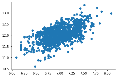
# 画出地上生活区面积与预测结果的关系图进行检验
plt.plot(np.expm1(test['GrLivArea']),result,'o')
[<matplotlib.lines.Line2D at 0x21638b44820>]

- 通过上图可知,房价与地上生活区面积成正相关,符合特征分析,所以预测结果合理。
# 保存数据
my_submission = pd.DataFrame({'Id':test.index,'SalePrice': result})
my_submission.to_csv('ex4-submission.csv', index=False)


 2万+
2万+

 被折叠的 条评论
为什么被折叠?
被折叠的 条评论
为什么被折叠?
 到【灌水乐园】发言


