使用BG/NBD模型与Gamma-Gamma模型预测客户的生命周期价值CLV/LTV

最新推荐文章于 2025-03-30 01:38:14 发布

吴下阿泽

最新推荐文章于 2025-03-30 01:38:14 发布

阅读量4.9k

点赞数 7

分类专栏：数据分析文章标签：数据分析 python 统计学

本文链接：https://blog.csdn.net/maiyida123/article/details/119832582

版权

数据分析专栏收录该内容

9 篇文章

订阅专栏

1. 背景

客户生命周期价值CLV: CLV是Customer Lifetime Value的简称，用来衡量一个客户（用户）在一段时期内对企业有多大价值，也称为LTV。

假如一个客户两年内在某商店内消费2000元，这2000元就是CLV,具有预测性。

CLV的常见作用：

预测用户还有多少价值、用以衡量投入产出比
在干预用户后，根据用户生命周期价值的变化，优化资源的投放。

那么如何计算CLV呢？我们可以使用BG/NBD模型预测客户的在指定时间内的交易次数，使用Gamma-Gamma模型预测在指定时间内的消费金额。

BG/NBD模型：BG/NBD模型又称为贝塔几何/负二项模型，用于描述非契约客户关系情境下重复购买行为。

该模型的几大假设：

用户在活跃状态下，一个用户在时间段t内完成的交易数量服从均值为λt的泊松分布
用户的交易率λ服从形状参数为r，逆尺度参数为α的gamma分布
每个用户在交易j完成后流失的概率服从参数为p(流失率)的几何分布
用户的流失率p服从形状参数为a，b的beta分布
每个用户的交易率λ和流失率p互相独立

Gamma-Gamma模型：BG/NBD模型只对客户存续时间和交易次数进行建模，并不涉及客户未来交易所带来的现金价值。而Gamma-Gamma模型就是对这个问题的一个扩展解决方案。

该模型的几大假设：

从客户角度上来说，交易金额在每个客户的平均交易价值上随机波动。(这一点并不是很有说服力)
所观察到的交易价值均值是隐含价值均值 𝐸(𝑀) 的非完美计量
交易价值均值在客户中是变化的，即使这个值是稳定的（这个假设非常大)
在客户中的平均交易价值的分布与交易过程无关。换句话说，就是现金价值与客户购买次数和客户存续时间可以分开建模。 (在真实场景下，这个假设很可能不成立)

关于两个模型的更多信息可以查看文末的参考链接，这里不做过多叙述。

本文通过使用Python的lifetimes包，使用上述的模型进行客户生命周期价值预测。

2. 案例

数据来源：数据为kaggle某零售销售数据

网盘点击下载
提取码：o5bk

2.1 数据整理与EDA

导入库

import numpy as np
import pandas as pd
from dateutil import relativedelta
from lifetimes import BetaGeoFitter, ModifiedBetaGeoFitter, GammaGammaFitter
from lifetimes.utils import summary_data_from_transaction_data
from sklearn.metrics import mean_squared_error
from lifetimes.plotting import plot_period_transactions, plot_frequency_recency_matrix 
import matplotlib.pyplot as plt
import seaborn as sns
plt.rcParams['font.sans-serif'] = ['SimHei'] 
plt.rcParams['axes.unicode_minus'] = False  
import warnings
warnings.filterwarnings("ignore")

数据加载预览

data = pd.read_csv('Retail_Data_Transactions.csv', parse_dates=['trans_date'])
data.head()

在这里插入图片描述

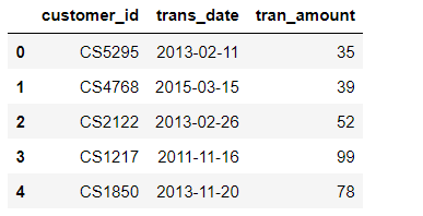
数据共三个列，客户id、交易日期、交易金额

查看数据格式

data.info()

在这里插入图片描述

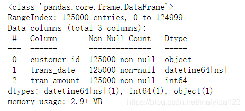
数据格式无需转换，并且没有空值

接下来对数据进行简单的探索性分析

查看客户的单次购买金额分布图

plt.subplots(figsize=(10,6))
data.tran_amount.hist()
plt.show()

在这里插入图片描述

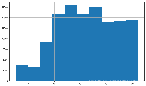
客户的单次购买金额集中分布在30-105之间。

查看客户购买总金额分布图

plt.subplots(figsize=(10,6))
data.groupby('customer_id').tran_amount.sum().hist(bins=20)
plt.show()

在这里插入图片描述

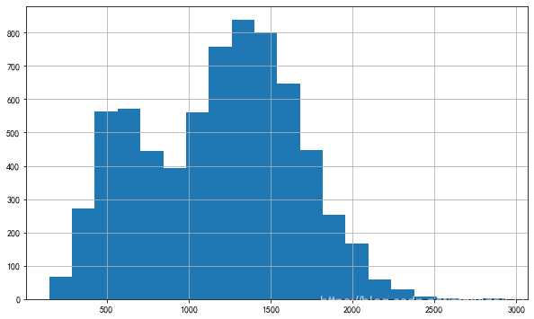
单个客户购买总金额呈现双峰分布，600与1300前后分布较多。

查看客户购买频次分布图

plt.subplots(figsize=(10,6))
data.groupby('customer_id').customer_id.count().hist(bins=20)
plt.show()

在这里插入图片描述

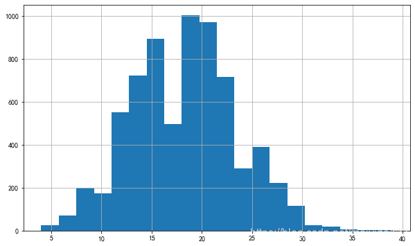
单个客户购买次数呈现双峰分布，15次与20次前后分布较多。

查看日购买金额时序分布图

fig, ax = plt.subplots(figsize=(20,5))
data.groupby('trans_date').agg({'tran_amount':'sum'}).plot(ax=ax)
plt.show()

在这里插入图片描述

没有明显的季节性变化，波动较为稳定

对于数据的分布有了大致的了解后，划分训练集测试集

# 以最后3个月为界划分训练集测试集
period_months = 3
date = data.trans_date.max() - relativedelta.relativedelta(months=period_months)
train = data[data.trans_date <= date]
test = data[data.trans_date > date]

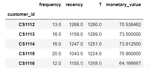
建模所需的数据：

frequency：表示客户重复购买的次数，比总购买量少一。如果以天为单位，第二天购买代表的是第一次重复，所以是购买天数-1。
T：表示客客户第一次购买到研究期结束之间的持续时间。
recency：表示客户第一次购买和最近一次购买之间的持续时间(因此，如果他们只进行了1次购买，则最近性为0。)
monetary_value：表示客户购买的平均价值。这等于客户的所有购买总额除以购买总数。请注意，此处的分母与上述frequency不同。

lifetimes有现成的函数计算这些数据，调用即可

train_df = summary_data_from_transaction_data(
    train,
    customer_id_col="customer_id",
    datetime_col="trans_date",
    monetary_value_col="tran_amount",
    freq="D",
)
train_df.head()

在这里插入图片描述
数据准备完毕，接下来开始建模。

2.2 BG/NBD 模型

2.2.1 建模

bgf = BetaGeoFitter(penalizer_coef=0.000001)  
bgf.fit(train_df['frequency'], train_df['recency'], train_df['T'])
bgf.summary

输出：
在这里插入图片描述
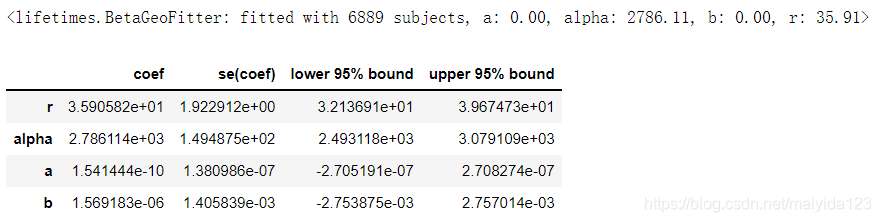
模型拟合出了所需参数: Gamma分布的 𝛼 和 𝑟 , Beta分布的 𝑎 和 𝑏 ，并给出了置信区间

2.2.2 预期交易的frequency /recency 可视化

预期未来三个月内的交易数量热力图

plt.subplots(figsize=(10,8))
plot_frequency_recency_matrix(bgf, T=90)  
plt.show()

在这里插入图片描述

由图我们可以看到，如果一个顾客已经购买了35次，而他们最近一次购买是在他们距离第一次购买1200天的时候，那么他们就是最好的顾客(右下角)。也就是在接下来的3个月内，他们购买概率高，预测的交易数最多。

最冷的客户是那些位于右上角的客户: 他们买得多，但我们已经很久没见到他们消费了。

客户留存热力图

plt.subplots(figsize=(10,8))
plot_probability_alive_matrix (bgf)
plt.show()

在这里插入图片描述
右上的客户以及深色带状的客户极可能已流失。

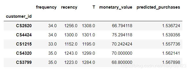
2.2.3 客户预期购买排行

在未来三个月内预期的客户购买数量排名

t = 90  # 90天
train_df['predicted_purchases'] = bgf.conditional_expected_number_of_purchases_up_to_time(t, train_df['frequency'], train_df['recency'], train_df['T'])
train_df.sort_values(by='predicted_purchases').tail(5)

在这里插入图片描述

2.2.4 模型拟合评估

2.2.4.1 可视化比较

查看其在训练集中的效果

fig, ax = plt.subplots(figsize=(10,6))
plot_period_transactions(bgf, max_frequency=60, ax=ax)
plt.show()

在这里插入图片描述
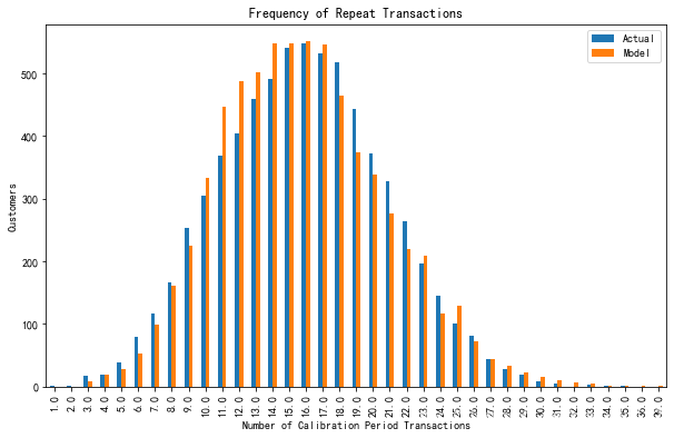
模型预测的交易次数和实际的交易次数对比，模型拟合效果看似还行

数据校准

使用测试集与训练集的预测结果对比

from lifetimes.utils import calibration_and_holdout_data
from lifetimes.plotting import plot_calibration_purchases_vs_holdout_purchases

summary_cal_holdout = calibration_and_holdout_data(data, 'customer_id', 'trans_date',
                                        calibration_period_end=train.trans_date.max(),
                                        observation_period_end=test.trans_date.max() )

fig, ax = plt.subplots(figsize=(10,6))
bgf.fit(summary_cal_holdout['frequency_cal'], 
        summary_cal_holdout['recency_cal'], 
        summary_cal_holdout['T_cal'])
plot_calibration_purchases_vs_holdout_purchases(bgf, summary_cal_holdout, n = 30,  ax=ax)
plt.show()

在这里插入图片描述

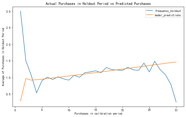
模型5-25次之间的预测与实际相近，前期低估，后期高估。

2.2.4.2 评估

数据整合

customers = train_df.reset_index()[['customer_id']]  
# 预测未来90天/3个月客户的购买次数
customers["pred_purchase_count"] = bgf.predict(
    90, train_df["frequency"], train_df["recency"], train_df["T"],
).values
# 统计测试集中的客户实际购买次数
test_count = test.groupby('customer_id').customer_id.count().rename('true_purchase_count').reset_index()
# 合并
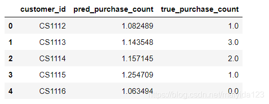
test_df = pd.merge(customers, test_count, on='customer_id', how='left')
# 如果有缺失值则填充为0
test_df.fillna(0, inplace=True)
# 预览
test_df.head()

在这里插入图片描述
查看预测值与实际值的基本统计信息

test_df.describe().round(3)

在这里插入图片描述

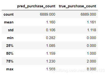
可以看到，模型预测的均值与实际均值相近，但高估了25%分位数之前的购买次数与高估了75%分位数之后的购买次数。

实际与预测的购买总次数比较

test_df[['pred_purchase_count', 'true_purchase_count']].sum().round()

在这里插入图片描述

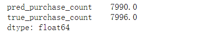
预测的总购买次数与实际相近

RMSE

print('RMSE: ', np.sqrt(mean_squared_error(test_df.true_purchase_count, test_df.pred_purchase_count)))

在这里插入图片描述

模型在个人层面的预测上还是存在不小的偏差。

2.3 Gamma-Gamma 模型

2.3.1 建模

查看平均购买金额和购买频率的相关性

train_df[['monetary_value', 'frequency']].corr()

在这里插入图片描述

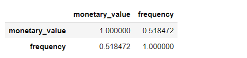
两者存在中等程度的相关性，这也预示着我们的结果不会太好，不过我们可以试试看

建模

预测未来三个月客户的平均交易价值

from lifetimes import GammaGammaFitter

ggf = GammaGammaFitter(penalizer_coef = 0.1)
ggf.fit(train_df['frequency'],
        train_df['monetary_value'])

ggf.conditional_expected_average_profit(train_df['frequency'],
        train_df['monetary_value']).head()

结果：
在这里插入图片描述
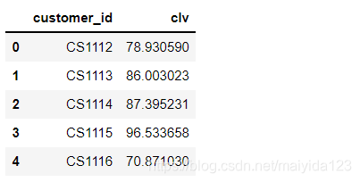
使用DCF现金流折现估算总价值

bgf.fit(train_df['frequency'], train_df['recency'], train_df['T'])

test_pred_amount = ggf.customer_lifetime_value(
        bgf, #the model to use to predict the number of future transactions
        train_df['frequency'],
        train_df['recency'],
        train_df['T'],
        train_df['monetary_value'],
        time=3, # months
        discount_rate=0.01 # monthly discount rate ~ 12.7% annually
).reset_index()

test_pred_amount.head()

在这里插入图片描述

2.3.2 评估

# 测试集中客户实际购买金额
test_amount = test.groupby('customer_id').tran_amount.sum().reset_index()
# 合并
test_amount_df = pd.merge(test_pred_amount, test_amount, on='customer_id', how='left')
# 缺失值填充
test_amount_df.fillna(0, inplace=True)
# 查看基本统计信息
test_amount_df.describe()

在这里插入图片描述

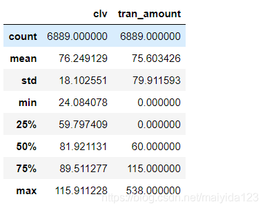
可以看到，模型预测的均值与实际均值相近，但预测的金额分布与实际有较大的偏差

查看购买总金额对比

test_amount_df[['tran_amount', 'clv']].sum()

在这里插入图片描述

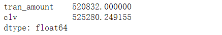
预测的客户购买总金额与实际值较为接近

RMSE

print('RMSE: ', np.sqrt(mean_squared_error(test_amount_df.tran_amount, test_amount_df.clv)))

在这里插入图片描述

预测值与实际值的偏差较大。

3. 结论

由于数据并不满足模型的假设要求，所以在个体预测上存在偏差，但是在总量上的预测与实际较为接近，可以作为宏观层面的一种参考。

参考：
lifetimes quickstart
用户增长 - BG/NBD概率模型预测用户生命周期LTV（二）