Layer Normalization (LN)

Briefing

Q: brief me on the key points of layer normalization, show me it's step by step implementation in python and give me some top rated links for further study

A (Bard): 

What it is:

• A technique for normalizing the activations of a neural network layer.
• Normalizes across features for each sample in a batch, rather than across the batch.
• Helps stabilize training, improve convergence, and prevent vanishing/exploding gradients.
• Often used in recurrent neural networks (RNNs) and transformers.

Key points:

• Normalization: Subtracts the mean and divides by the standard deviation for each feature within a sample.
• Independence from batch size: Works effectively even with small batch sizes.
• No dependency between training cases: Doesn't introduce new dependencies between samples.
• Benefits: Improves training speed, generalization, and stability.

Implementation provided uses keras, hence skipped.

Top-rated links for further study:

• Original paper: https://arxiv.org/abs/1607.06450
• TensorFlow documentation: https://www.tensorflow.org/api_docs/python/tf/keras/layers/LayerNormalization
• Keras documentation: LayerNormalization layer
• Pinecone explanation: Build Better Deep Learning Models with Batch and Layer Normalization | Pinecone
• Papers With Code overview: Layer Normalization Explained | Papers With Code

here on I use the Pinecore article as main source, as it's the more comprehensive and easily read one.

VS. Batch Normalization (BN)

as you can read from the abstract of the original paper,

Training state-of-the-art, deep neural networks is computationally expensive. One way to reduce the training time is to normalize the activities of the neurons. A recently introduced technique called batch normalization uses the distribution of the summed input to a neuron over a mini-batch of training cases to compute a mean and variance which are then used to normalize the summed input to that neuron on each training case. This significantly reduces the training time in feed-forward neural networks. However, the effect of batch normalization is dependent on the mini-batch size and it is not obvious how to apply it to recurrent neural networks. In this paper, we transpose batch normalization into layer normalization by computing the mean and variance used for normalization from all of the summed inputs to the neurons in a layer on a single training case. Like batch normalization, we also give each neuron its own adaptive bias and gain which are applied after the normalization but before the non-linearity. Unlike batch normalization, layer normalization performs exactly the same computation at training and test times. It is also straightforward to apply to recurrent neural networks by computing the normalization statistics separately at each time step. Layer normalization is very effective at stabilizing the hidden state dynamics in recurrent networks. Empirically, we show that layer normalization can substantially reduce the training time compared with previously published techniques.

LN is proposed as an alternative or complement to BN, hence it's best to start with a solid understanding of BN.

here is an article I collected about BN: 

Batch Normalization: Basics and Intuition_what shuld we choose-CSDN博客

the recommended paper with code link has a nice visualization about the "transpose" induced-difference

main source would also feature a section dedicated to BN.  

Main Source

Why Any Regularization

Even with the optimal model architecture, how the model is trained can make the difference between a phenomenal success or a scorching failure.

For example, take weight initialization: In the process of training a neural network, we initialize the weights which are then updated as the training proceeds. For a certain random initialization, the outputs from one or more of the intermediate layers can be abnormally large. This leads to instability in the training process, which means the network will not learn anything useful during training.

Batch and layer normalization are two strategies for training neural networks faster, without having to be overly cautious with initialization and other regularization techniques.

When you train a neural network on a dataset, the numeric input features could take on values in potentially different ranges. For example, if you’re working with a dataset of student loans with the age of the student and the tuition as two input features, the two values are on totally different scales. While the age of a student will have a median value in the range 18 to 25 years, the tuition could take on values in the range $20K - $50K for a given academic year.

If you proceed to train your model on such datasets with input features on different scales, you’ll notice that the neural network takes significantly longer to train because the gradient descent algorithm takes longer to converge when the input features are not all on the same scale. Additionally, such high values can also propagate through the layers of the network leading to the accumulation of large error gradients that make the training process unstable, called the problem of exploding gradients.

To overcome the above-mentioned issues of longer training time and instability, you should consider preprocessing your input data ahead of training. Preprocessing techniques such as normalization and standardization transform the input data to be on the same scale.

Normalization vs Standardization

Normalization works by mapping all values of a feature to be in the range [0,1] using the transformation:

                                        

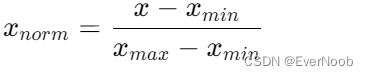
Standardization, on the other hand, transforms the input values such that they follow a distribution with zero mean and unit variance. Mathematically, the transformation on the data points in a distribution with mean μ and standard deviation σ is given by:

                        ​​​​​​​        ​​​​​​​        ​​​​​​​        ​​​​​​​        

In practice, this process of standardization is also referred to as normalization (not to be confused with the normalization process discussed above).

==> while for a procedure where we produce a set of values that lie between 0 and 1, summing to 1, it's called normalizing to a probability distribution. An example is softmax, though it not only normalizes values to sum to 1 but also emphasizes the largest values and suppresses smaller ones. This makes it particularly useful in tasks where distinguishing the most likely outcomes is crucial, such as in classification problems.

Batch Normalization

Why

For a network with hidden layers, the output of layer k-1 serves as the input to layer k. If the inputs to a particular layer change drastically, we can again run into the problem of unstable gradients.

When working with large datasets, you’ll split the dataset into multiple batches and run the mini-batch gradient descent. The mini-batch gradient descent algorithm optimizes the parameters of the neural network by batchwise processing of the dataset, one batch at a time.

It’s also possible that the input distribution at a particular layer keeps changing across batches. The seminal paper titled Batch Normalization: Accelerating Deep Network Training by Reducing Internal Covariate Shift by Sergey Ioffe and Christian Szegedy refers to this change in distribution of the input to a particular layer across batches as internal covariate shift. For instance, if the distribution of data at the input of layer K keeps changing across batches, the network will take longer to train.

But why does this hamper the training process?

For each batch in the input dataset, the mini-batch gradient descent algorithm runs its updates. It updates the weights and biases (parameters) of the neural network so as to fit to the distribution seen at the input to the specific layer for the current batch.

Now that the network has learned to fit to the current distribution, if the distribution changes substantially for the next batch, it now has to update the parameters to fit to the new distribution. This slows down the training process.

However, if we transpose the idea of normalizing the inputs to the hidden layers in the network, we can potentially overcome the limitations imposed by exploding activations and fluctuating distributions at the layer’s input. Batch normalization helps us achieve this, one mini-batch at a time, to accelerate the training process.

What

For any hidden layer h, we pass the inputs through a non-linear activation to get the output. For every neuron (activation) in a particular layer, we can force the pre-activations to have zero mean and unit standard deviation. This can be achieved by subtracting the mean from each of the input features across the mini-batch and dividing by the standard deviation.

Following the output of the layer k-1, we can add a layer that performs this normalization operation across the mini-batch so that the pre-activations at layer k are unit Gaussians. The figure below illustrates this.

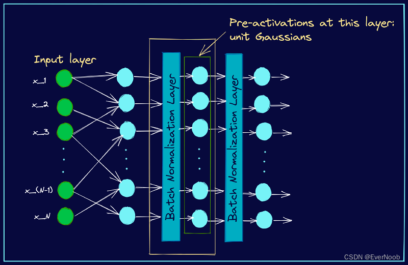
Section of a Neural Network with Batch Normalization Layer (Image by the author, Bala Priya C)

==> consider the suffix to x to be the mini batch indices.

As an example, let’s consider a mini-batch with 3 input samples, each input vector being four features long. Here’s a simple illustration of how the mean and standard deviation are computed in this case. Once we compute the mean and standard deviation, we can subtract the mean and divide by the standard deviation.

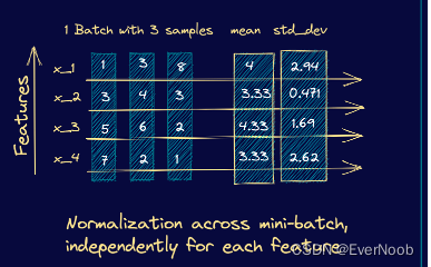
How Batch Normalization Works - An Example (Image by the author, Bala Priya C)

==> for the above illustration, though, obvously the suffices of x are feature indices.

However, forcing all the pre-activations to be zero and unit standard deviation across all batches can be too restrictive. It may be the case that the fluctuant distributions are necessary for the network to learn certain classes better.

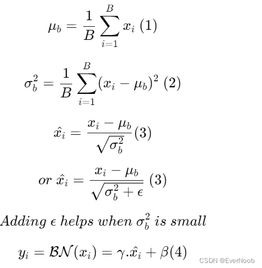
To address this, batch normalization introduces two parameters: a scaling factor gamma (γ) and an offset beta (β). These are learnable parameters, so if the fluctuation in input distribution is necessary for the neural network to learn a certain class better, then the network learns the optimal values of gamma and beta for each mini-batch. The gamma and beta are learnable such that it’s possible to go back from the normalized pre-activations to the actual distributions that the pre-activations follow.

Putting it all together, we have the following steps for batch normalization. If x(k) is the pre-activation corresponding to the k-th neuron in a layer, we denote it by x to simplify notation.

Limitations

Two limitations of batch normalization can arise:

• In batch normalization, we use the batch statistics: the mean and standard deviation corresponding to the current mini-batch. However, when the batch size is small, the sample mean and sample standard deviation are not representative enough of the actual distribution and the network cannot learn anything meaningful.
• As batch normalization depends on batch statistics for normalization, it is less suited for sequence models. This is because, in sequence models, we may have sequences of potentially different lengths and smaller batch sizes corresponding to longer sequences.

For convolutional neural networks (ConvNets), batch normalization is still recommended for faster training.

Layer Normalization

What

Layer Normalization was proposed by researchers Jimmy Lei Ba, Jamie Ryan Kiros, and Geoffrey E. Hinton. In layer normalization, all neurons in a particular layer effectively have the same distribution across all features for a given input.

For example, if each input has d features, it’s a d-dimensional vector. If there are B elements in a batch, the normalization is done along the length of the d-dimensional vector and not across the batch of size B.

==> the definition is by itself quie clear, however, we still do need to heed what we regard as feature in communication; by the paper with code's illustration, d = H*W*C, however, under different context, we can also have N = 1, while we define batch size to be H*W, and feature length to be C.

Normalizing across all features but for each of the inputs to a specific layer removes the dependence on batches. This makes layer normalization well suited for sequence models such as transformers and recurrent neural networks (RNNs) that were popular in the pre-transformer era.

Here’s an example showing the computation of the mean and variance for layer normalization. We consider the example of a mini-batch containing three input samples, each with four features.

How Layer Normalization Works - An Example (Image by the author)

From these steps, we see that they’re similar to the steps we had in batch normalization. However, instead of the batch statistics, we use the mean and variance corresponding to specific input to the neurons in a particular layer, say k. This is equivalent to normalizing the output vector from the layer k-1.

Batch Normalization vs Layer Normalization

So far, we learned how batch and layer normalization work. Let’s summarize the key differences between the two techniques.

• Batch normalization normalizes each feature independently across the mini-batch. Layer normalization normalizes each of the inputs in the batch independently across all features.
• As batch normalization is dependent on batch size, it’s not effective for small batch sizes. Layer normalization is independent of the batch size, so it can be applied to batches with smaller sizes as well.
• Batch normalization requires different processing at training and inference times. As layer normalization is done along the length of input to a specific layer, the same set of operations can be used at both training and inference times.