消噪的Diffusion扩散模型

最新推荐文章于 2024-05-25 16:20:21 发布

murongmeng

最新推荐文章于 2024-05-25 16:20:21 发布

阅读量1.7k

点赞数 19

文章标签：人工智能

本文链接：https://blog.csdn.net/murongmeng/article/details/133249705

版权

1. 环境准备

进入案例官网, 本体验的所有代码都来自mindspore官网：

MindSporehttps://www.mindspore.cn/tutorials/application/zh-CN/r2.1/generative/diffusion.html点击”在ModelArts平台运行“

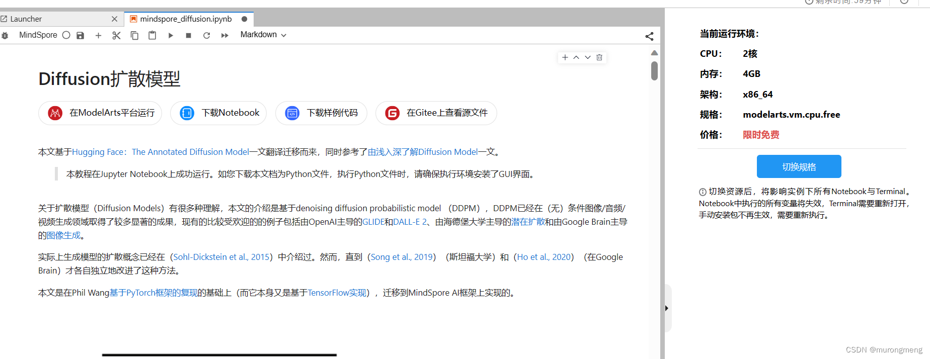
进入modelArts平台

免费的CPU 2核4GB

有多种选择：

2. Diffusion扩散模型介绍

本文对Diffusion扩散模型的理解是基于DDPM，而DDPM已经在（无）条件图像/音频/视频生成领域取得了较多显著的成果，现有的比较受欢迎的的例子包括由OpenAI主导的GLIDE和DALL-E 2、由海德堡大学主导的潜在扩散和由Google Brain主导的图像生成。

将Diffusion与其他生成模型（如Normalizing Flows、GAN或VAE）进行比较，它们都将噪声从一些简单分布转换为数据样本，Diffusion也是从纯噪声开始通过一个神经网络学习逐步去噪，最终得到一个实际图像。 Diffusion基于马尔科夫链，对于图像的处理包括以下两个过程：

正向扩散过程 q：它逐渐将高斯噪声添加到图像中，直到最终得到纯噪声

反向去噪的扩散过程 pθ：通过训练神经网络从纯噪声开始逐渐对图像去噪，直到最终得到一个实际的图像

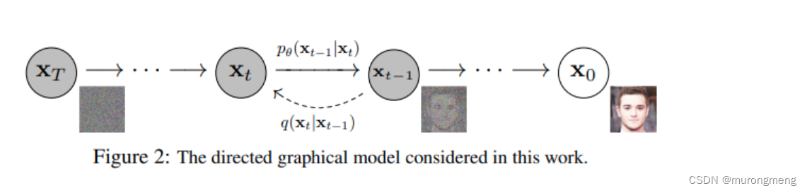
如图所示：X0-Xt的过程是Diffusion的前向过程，每一步的随机过程为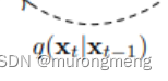：， Xt-X0的过程为Diffusion的逆向过程，每一步的随机过程为：

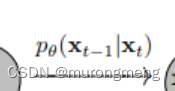
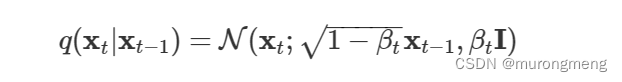
Diffusion 前向过程

Diffusion 前向过程就是图片加噪声的过程，也叫做马尔科夫过程：

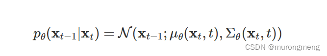
Diffusion 逆向过程

Diffusion 逆向过程是去噪过程，通过神经网络学习并表示 pθ(xt−1|xt) 的过程就是Diffusion 逆向去噪的核心，公式是：

3. 体验实验

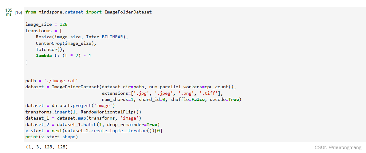
实验开始之前请确保安装并导入所需的库（假设您已经安装了MindSpore、download、dataset、matplotlib以及tqdm）

不过此次体验用的是官网modelarts直接用mindspore_diffusion.ipynb运行，不需要再次安装

点击左上角的运行即可

构建Diffusion模型

定义了一些帮助函数和类，这些函数和类将在实现神经网络时使用。

def rearrange(head, inputs):
    b, hc, x, y = inputs.shape
    c = hc // head
    return inputs.reshape((b, head, c, x * y))

def rsqrt(x):
    res = ops.sqrt(x)
    return ops.inv(res)

def randn_like(x, dtype=None):
    if dtype is None:
        dtype = x.dtype
    res = ops.standard_normal(x.shape).astype(dtype)
    return res

def randn(shape, dtype=None):
    if dtype is None:
        dtype = ms.float32
    res = ops.standard_normal(shape).astype(dtype)
    return res

def randint(low, high, size, dtype=ms.int32):
    res = ops.uniform(size, Tensor(low, dtype), Tensor(high, dtype), dtype=dtype)
    return res

def exists(x):
    return x is not None

def default(val, d):
    if exists(val):
        return val
    return d() if callable(d) else d

def _check_dtype(d1, d2):
    if ms.float32 in (d1, d2):
        return ms.float32
    if d1 == d2:
        return d1
    raise ValueError('dtype is not supported.')

class Residual(nn.Cell):
    def __init__(self, fn):
        super().__init__()
        self.fn = fn

    def construct(self, x, *args, **kwargs):
        return self.fn(x, *args, **kwargs) + x

上采样和下采样操作的别名

位置向量

SinusoidalPositionEmbeddings模块采用(batch_size, 1)形状的张量作为输入（即批处理中几个有噪声图像的噪声水平），并将其转换为(batch_size, dim)形状的张量，其中dim是位置嵌入的尺寸。然后，我们将其添加到每个剩余块中。

ResNet/ConvNeXT块

因为Phil Wang决定添加ConvNeXT替换ResNet，在图像领域取得巨大成功，因此本文选择ConvNeXT块构建U-Net模型

class Block(nn.Cell):
    def __init__(self, dim, dim_out, groups=1):
        super().__init__()
        self.proj = nn.Conv2d(dim, dim_out, 3, pad_mode="pad", padding=1)
        self.proj = c(dim, dim_out, 3, padding=1, pad_mode='pad')
        self.norm = nn.GroupNorm(groups, dim_out)
        self.act = nn.SiLU()

    def construct(self, x, scale_shift=None):
        x = self.proj(x)
        x = self.norm(x)

        if exists(scale_shift):
            scale, shift = scale_shift
            x = x * (scale + 1) + shift

        x = self.act(x)
        return x

class ConvNextBlock(nn.Cell):
    def __init__(self, dim, dim_out, *, time_emb_dim=None, mult=2, norm=True):
        super().__init__()
        self.mlp = (
            nn.SequentialCell(nn.GELU(), nn.Dense(time_emb_dim, dim))
            if exists(time_emb_dim)
            else None
        )

        self.ds_conv = nn.Conv2d(dim, dim, 7, padding=3, group=dim, pad_mode="pad")
        self.net = nn.SequentialCell(
            nn.GroupNorm(1, dim) if norm else nn.Identity(),
            nn.Conv2d(dim, dim_out * mult, 3, padding=1, pad_mode="pad"),
            nn.GELU(),
            nn.GroupNorm(1, dim_out * mult),
            nn.Conv2d(dim_out * mult, dim_out, 3, padding=1, pad_mode="pad"),
        )

        self.res_conv = nn.Conv2d(dim, dim_out, 1) if dim != dim_out else nn.Identity()

    def construct(self, x, time_emb=None):
        h = self.ds_conv(x)
        if exists(self.mlp) and exists(time_emb):
            assert exists(time_emb), "time embedding must be passed in"
            condition = self.mlp(time_emb)
            condition = condition.expand_dims(-1).expand_dims(-1)
            h = h + condition

        h = self.net(h)
        return h + self.res_conv(x)

Attention模块

定义SiLU模块，DDPM作者将其添加到卷积块之间。SiLU是著名的Transformer架构，在人工智能的各个领域都取得了巨大的成功，从NLP到蛋白质折叠。

class Attention(nn.Cell):
    def __init__(self, dim, heads=4, dim_head=32):
        super().__init__()
        self.scale = dim_head ** -0.5
        self.heads = heads
        hidden_dim = dim_head * heads

        self.to_qkv = nn.Conv2d(dim, hidden_dim * 3, 1, pad_mode='valid', has_bias=False)
        self.to_out = nn.Conv2d(hidden_dim, dim, 1, pad_mode='valid', has_bias=True)
        self.map = ops.Map()
        self.partial = ops.Partial()

    def construct(self, x):
        b, _, h, w = x.shape
        qkv = self.to_qkv(x).chunk(3, 1)
        q, k, v = self.map(self.partial(rearrange, self.heads), qkv)

        q = q * self.scale

        # 'b h d i, b h d j -> b h i j'
        sim = ops.bmm(q.swapaxes(2, 3), k)
        attn = ops.softmax(sim, axis=-1)
        # 'b h i j, b h d j -> b h i d'
        out = ops.bmm(attn, v.swapaxes(2, 3))
        out = out.swapaxes(-1, -2).reshape((b, -1, h, w))

        return self.to_out(out)


class LayerNorm(nn.Cell):
    def __init__(self, dim):
        super().__init__()
        self.g = Parameter(initializer('ones', (1, dim, 1, 1)), name='g')

    def construct(self, x):
        eps = 1e-5
        var = x.var(1, keepdims=True)
        mean = x.mean(1, keep_dims=True)
        return (x - mean) * rsqrt((var + eps)) * self.g


class LinearAttention(nn.Cell):
    def __init__(self, dim, heads=4, dim_head=32):
        super().__init__()
        self.scale = dim_head ** -0.5
        self.heads = heads
        hidden_dim = dim_head * heads
        self.to_qkv = nn.Conv2d(dim, hidden_dim * 3, 1, pad_mode='valid', has_bias=False)

        self.to_out = nn.SequentialCell(
            nn.Conv2d(hidden_dim, dim, 1, pad_mode='valid', has_bias=True),
            LayerNorm(dim)
        )

        self.map = ops.Map()
        self.partial = ops.Partial()

    def construct(self, x):
        b, _, h, w = x.shape
        qkv = self.to_qkv(x).chunk(3, 1)
        q, k, v = self.map(self.partial(rearrange, self.heads), qkv)

        q = ops.softmax(q, -2)
        k = ops.softmax(k, -1)

        q = q * self.scale
        v = v / (h * w)

        # 'b h d n, b h e n -> b h d e'
        context = ops.bmm(k, v.swapaxes(2, 3))
        # 'b h d e, b h d n -> b h e n'
        out = ops.bmm(context.swapaxes(2, 3), q)

        out = out.reshape((b, -1, h, w))
        return self.to_out(out)

组归一化

下面，我们定义一个PreNorm类，将用于在注意层之前应用groupnorm。

条件U-Net

上面定义了所有的构建块（位置嵌入、ResNet/ConvNeXT块、Attention和组归一化），下面开始定义整个神经网络

网络构建过程如下：

将卷积层应用于噪声图像批上，并计算噪声水平的位置
应用一系列下采样级。每个下采样阶段由2个ResNet/ConvNeXT块 + groupnorm + attention + 残差连接 + 一个下采样操作组成
在网络的中间，再次应用ResNet或ConvNeXT块，并与attention交织
应用一系列上采样级。每个上采样级由2个ResNet/ConvNeXT块+ groupnorm + attention + 残差连接 + 一个上采样操作组成
应用ResNet/ConvNeXT块，然后应用卷积层

class Unet(nn.Cell):
    def __init__(
            self,
            dim,
            init_dim=None,
            out_dim=None,
            dim_mults=(1, 2, 4, 8),
            channels=3,
            with_time_emb=True,
            convnext_mult=2,
    ):
        super().__init__()

        self.channels = channels

        init_dim = default(init_dim, dim // 3 * 2)
        self.init_conv = nn.Conv2d(channels, init_dim, 7, padding=3, pad_mode="pad", has_bias=True)

        dims = [init_dim, *map(lambda m: dim * m, dim_mults)]
        in_out = list(zip(dims[:-1], dims[1:]))

        block_klass = partial(ConvNextBlock, mult=convnext_mult)

        if with_time_emb:
            time_dim = dim * 4
            self.time_mlp = nn.SequentialCell(
                SinusoidalPositionEmbeddings(dim),
                nn.Dense(dim, time_dim),
                nn.GELU(),
                nn.Dense(time_dim, time_dim),
            )
        else:
            time_dim = None
            self.time_mlp = None

        self.downs = nn.CellList([])
        self.ups = nn.CellList([])
        num_resolutions = len(in_out)

        for ind, (dim_in, dim_out) in enumerate(in_out):
            is_last = ind >= (num_resolutions - 1)

            self.downs.append(
                nn.CellList(
                    [
                        block_klass(dim_in, dim_out, time_emb_dim=time_dim),
                        block_klass(dim_out, dim_out, time_emb_dim=time_dim),
                        Residual(PreNorm(dim_out, LinearAttention(dim_out))),
                        Downsample(dim_out) if not is_last else nn.Identity(),
                    ]
                )
            )

        mid_dim = dims[-1]
        self.mid_block1 = block_klass(mid_dim, mid_dim, time_emb_dim=time_dim)
        self.mid_attn = Residual(PreNorm(mid_dim, Attention(mid_dim)))
        self.mid_block2 = block_klass(mid_dim, mid_dim, time_emb_dim=time_dim)

        for ind, (dim_in, dim_out) in enumerate(reversed(in_out[1:])):
            is_last = ind >= (num_resolutions - 1)

            self.ups.append(
                nn.CellList(
                    [
                        block_klass(dim_out * 2, dim_in, time_emb_dim=time_dim),
                        block_klass(dim_in, dim_in, time_emb_dim=time_dim),
                        Residual(PreNorm(dim_in, LinearAttention(dim_in))),
                        Upsample(dim_in) if not is_last else nn.Identity(),
                    ]
                )
            )

        out_dim = default(out_dim, channels)
        self.final_conv = nn.SequentialCell(
            block_klass(dim, dim), nn.Conv2d(dim, out_dim, 1)
        )

    def construct(self, x, time):
        x = self.init_conv(x)

        t = self.time_mlp(time) if exists(self.time_mlp) else None

        h = []

        for block1, block2, attn, downsample in self.downs:
            x = block1(x, t)
            x = block2(x, t)
            x = attn(x)
            h.append(x)

            x = downsample(x)

        x = self.mid_block1(x, t)
        x = self.mid_attn(x)
        x = self.mid_block2(x, t)

        len_h = len(h) - 1
        for block1, block2, attn, upsample in self.ups:
            x = ops.concat((x, h[len_h]), 1)
            len_h -= 1
            x = block1(x, t)
            x = block2(x, t)
            x = attn(x)

            x = upsample(x)
        return self.final_conv(x)

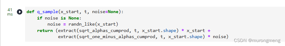
正向扩散

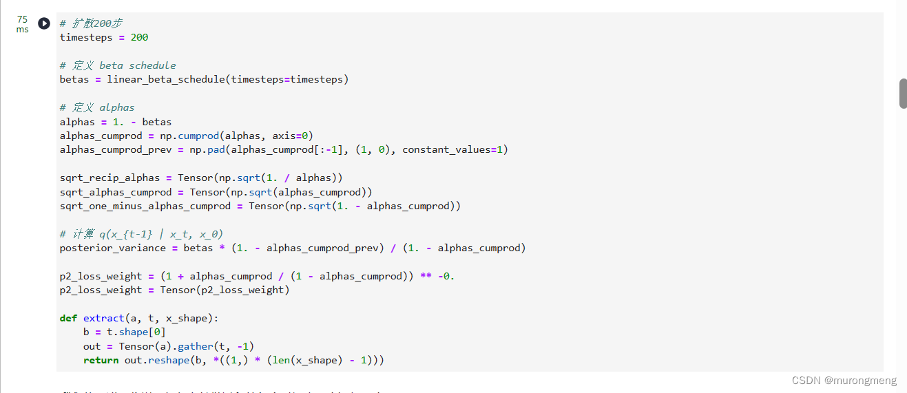
定义T时间步的时间表：

使用T=200时间步长的线性计划

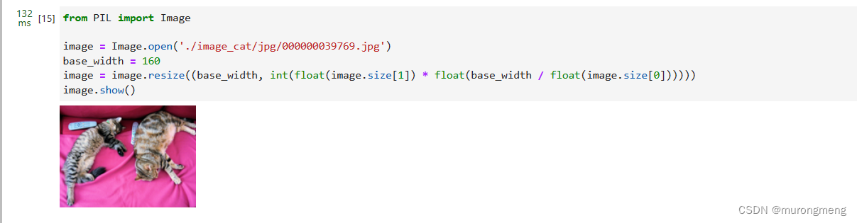
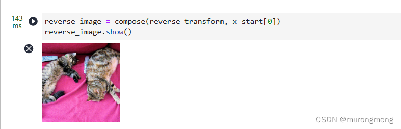
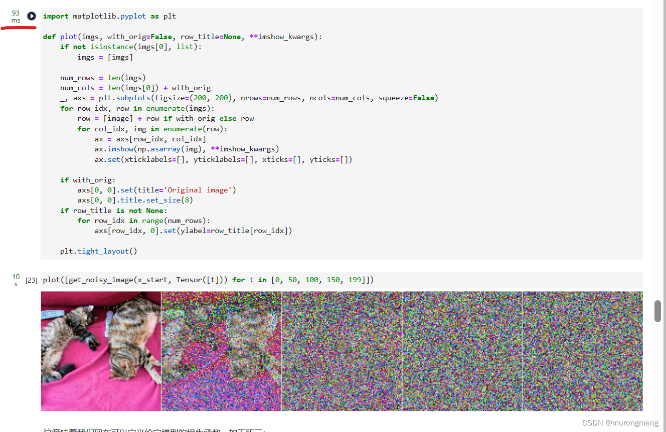
数据的话，使用的是猫图像来说明如何在扩散过程的每个时间步骤中添加噪音

# 下载猫猫图像
url = 'https://mindspore-website.obs.cn-north-4.myhuaweicloud.com/notebook/datasets/image_cat.zip'
path = download(url, './', kind="zip", replace=True)

from PIL import Image

image = Image.open('./image_cat/jpg/000000039769.jpg')
base_width = 160
image = image.resize((base_width, int(float(image.size[1]) * float(base_width / float(image.size[0])))))
image.show()

噪声被添加到mindspore张量中，而不是Pillow图像。我们将首先定义图像转换，允许我们从PIL图像转换到mindspore张量（我们可以在其上添加噪声），反之亦然。

这些转换相当简单：我们首先通过除以255来标准化图像（使它们在 [0,1]范围内），然后确保它们在 [−1,1]范围内。

定义了反向变换，它接收一个包含 [−1,1]中的张量，并将它们转回 PIL 图像：

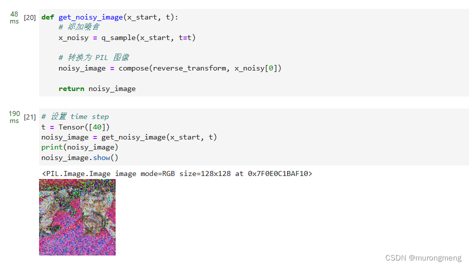
验证结果：

定义前向扩散过程：

在特定的步长上测试它，下面是可视化结果：

不同的时间步骤可视化此情况

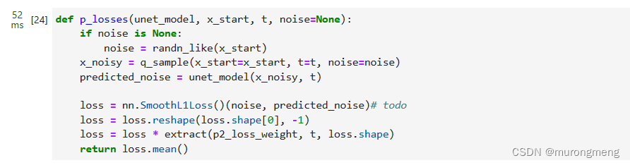
定义给定模型的损失函数，denoise_model将是我们上面定义的U-Net。我们将在真实噪声和预测噪声之间使用Huber损失

数据准备与处理

下载并解压Fashion_MNIST数据集到指定路径，此数据集由已经具有相同分辨率的图像组成，即28x28

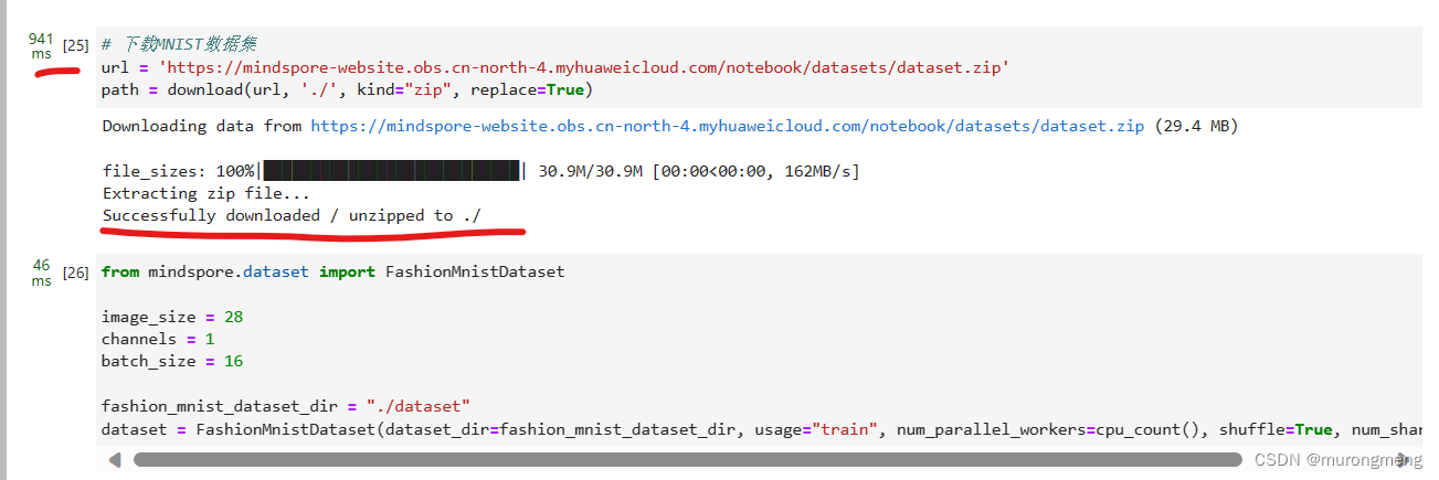
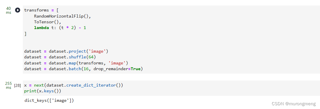
定义一个transform操作，将在整个数据集上动态应用该操作。该操作应用一些基本的图像预处理：随机水平翻转、重新调整，最后使它们的值在 [−1,1][−1,1] 范围内。

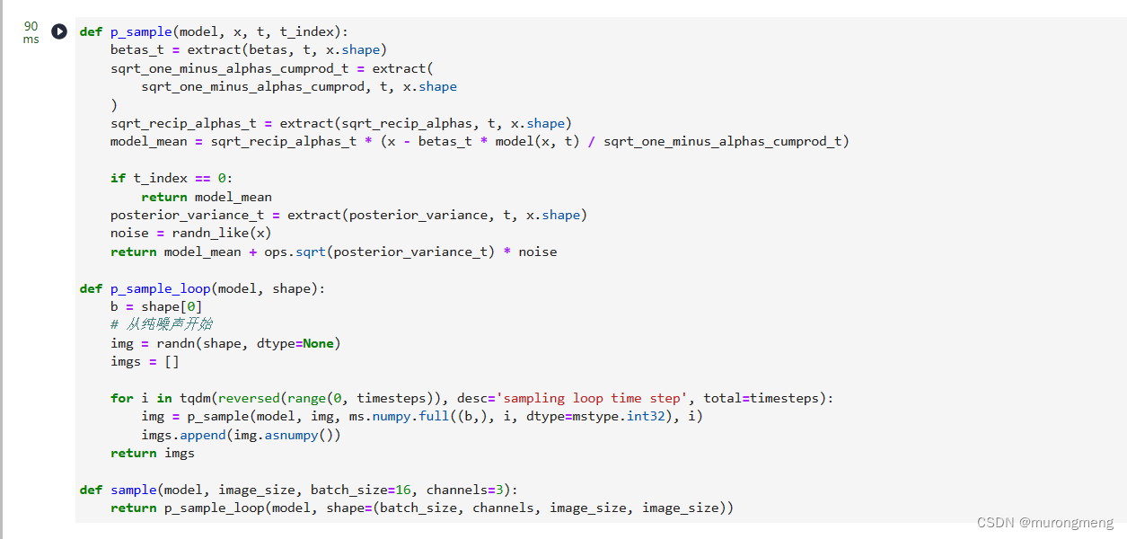
采样

采样算法：

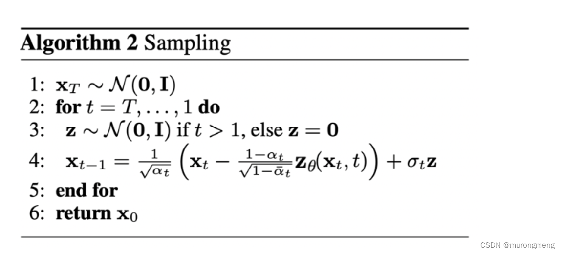
理想情况下，我们最终会得到一个看起来像是来自真实数据分布的图像

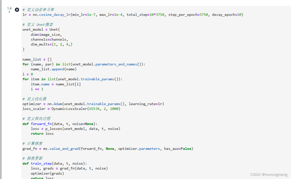
训练过程

# 定义动态学习率
lr = nn.cosine_decay_lr(min_lr=1e-7, max_lr=1e-4, total_step=10*3750, step_per_epoch=3750, decay_epoch=10)

# 定义 Unet模型
unet_model = Unet(
    dim=image_size,
    channels=channels,
    dim_mults=(1, 2, 4,)
)

name_list = []
for (name, par) in list(unet_model.parameters_and_names()):
    name_list.append(name)
i = 0
for item in list(unet_model.trainable_params()):
    item.name = name_list[i]
    i += 1

# 定义优化器
optimizer = nn.Adam(unet_model.trainable_params(), learning_rate=lr)
loss_scaler = DynamicLossScaler(65536, 2, 1000)

# 定义前向过程
def forward_fn(data, t, noise=None):
    loss = p_losses(unet_model, data, t, noise)
    return loss

# 计算梯度
grad_fn = ms.value_and_grad(forward_fn, None, optimizer.parameters, has_aux=False)

# 梯度更新
def train_step(data, t, noise):
    loss, grads = grad_fn(data, t, noise)
    optimizer(grads)
    return loss

import time

epochs = 10

for epoch in range(epochs):
    begin_time = time.time()
    for step, batch in enumerate(dataset.create_tuple_iterator()):
        unet_model.set_train()
        batch_size = batch[0].shape[0]
        t = randint(0, timesteps, (batch_size,), dtype=ms.int32)
        noise = randn_like(batch[0])
        loss = train_step(batch[0], t, noise)

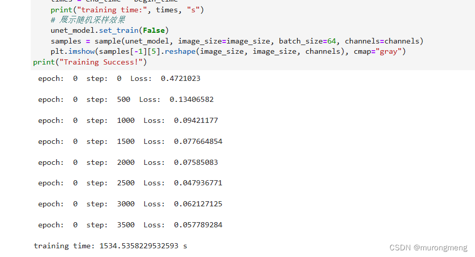
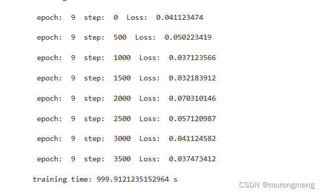
        if step % 500 == 0:
            print(" epoch: ", epoch, " step: ", step, " Loss: ", loss)
    end_time = time.time()
    times = end_time - begin_time
    print("training time:", times, "s")
    # 展示随机采样效果
    unet_model.set_train(False)
    samples = sample(unet_model, image_size=image_size, batch_size=64, channels=channels)
    plt.imshow(samples[-1][5].reshape(image_size, image_size, channels), cmap="gray")
print("Training Success!")

训练数据：

推理过程（从模型中采样）

# 采样64个图片
unet_model.set_train(False)
samples = sample(unet_model, image_size=image_size, batch_size=64, channels=channels)

# 展示一个随机效果
random_index = 5
plt.imshow(samples[-1][random_index].reshape(image_size, image_size, channels), cmap="gray")

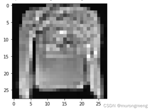
可以看到这个模型能产生一件衣服！

请注意，我们训练的数据集分辨率相当低（28x28）。

我们还可以创建去噪过程的gif：

import matplotlib.animation as animation

random_index = 53

fig = plt.figure()
ims = []
for i in range(timesteps):
    im = plt.imshow(samples[i][random_index].reshape(image_size, image_size, channels), cmap="gray", animated=True)
    ims.append([im])

animate = animation.ArtistAnimation(fig, ims, interval=50, blit=True, repeat_delay=100)
animate.save('diffusion.gif')
plt.show()

murongmeng

关注

19
点赞
踩
27

收藏

觉得还不错? 一键收藏
1
评论
消噪的Diffusion扩散模型

本文对Diffusion扩散模型的理解是基于DDPM，而DDPM已经在（无）条件图像/音频/视频生成领域取得了较多显著的成果，现有的比较受欢迎的的例子包括由OpenAI主导的GLIDE和DALL-E 2、由海德堡大学主导的潜在扩散和由Google Brain主导的图像生成。将Diffusion与其他生成模型（如Normalizing Flows、GAN或VAE）进行比较，它们都将噪声从一些简单分布转换为数据样本，Diffusion也是从纯噪声开始通过一个神经网络学习逐步去噪，最终得到一个实际图像。
复制链接

扫一扫