3、目标跟踪：数据关联

---

一、数据关联简介

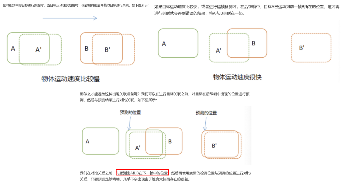
• The MOT problem can be viewed as a data association problem where the aim is to associate detections across frames in a video sequence
• 为什么不使用前后两帧的检测结果直接进行匹配呢？1、速度快了可能误匹配，2、存在漏检的情况（此时 kf 还能继续预测，只用检测则丢失了 track 当前帧的信息）

import numpy as np
from scipy.optimize import linear_sum_assignment


"""在这里我们对检测框和跟踪框进行匹配，整个流程是遍历检测框和跟踪框，
并进行匹配，匹配成功的将其保留，未成功的将其删除"""
def associate_detections_to_trackers(detections, trackers, iou_threshold=0.3):
    """
    将检测框bbox与卡尔曼滤波器的跟踪框进行关联匹配
    :param detections:检测框
    :param trackers:跟踪框，即跟踪目标
    :param iou_threshold:IOU阈值
    :return:跟踪成功目标的矩阵：matchs
            新增目标的矩阵：unmatched_detections
            跟踪失败即离开画面的目标矩阵：unmatched_trackers
    """
    # 跟踪目标数量为0，直接构造结果
    if (len(trackers) == 0) or (len(detections) == 0):
        return np.empty((0, 2), dtype=int), np.arange(len(detections)), np.empty((0, 5), dtype=int)

    # iou 不支持数组计算。逐个计算两两间的交并比，调用 linear_assignment 进行匹配
    iou_matrix = np.zeros((len(detections), len(trackers)), dtype=np.float32)
    # 遍历目标检测的 bbox 集合，每个检测框的标识为 d
    for d, det in enumerate(detections):
        # 遍历跟踪框（卡尔曼滤波器预测）bbox 集合，每个跟踪框标识为 t
        for t, trk in enumerate(trackers):
            iou_matrix[d, t] = iou(det, trk)
    # 通过匈牙利算法将跟踪框和检测框以 [[d,t]...] 的二维矩阵的形式存储在 match_indices 中
    result = linear_sum_assignment(-iou_matrix)
    matched_indices = np.array(list(zip(*result)))

    # 记录未匹配的检测框及跟踪框
    # 未匹配的检测框放入 unmatched_detections 中，表示有新的目标进入画面，要新增跟踪器跟踪目标
    unmatched_detections = []
    for d, det in enumerate(detections):
        if d not in matched_indices[:, 0]:
            unmatched_detections.append(d)
    # 未匹配的跟踪框放入 unmatched_trackers 中，表示目标离开之前的画面，应删除对应的跟踪器
    unmatched_trackers = []
    for t, trk in enumerate(trackers):
        if t not in matched_indices[:, 1]:
            unmatched_trackers.append(t)
    # 将匹配成功的跟踪框放入 matches 中
    matches = []
    for m in matched_indices:
        # 过滤掉 IOU 低的匹配，将其放入到 unmatched_detections 和 unmatched_trackers
        if iou_matrix[m[0], m[1]] < iou_threshold:
            unmatched_detections.append(m[0])
            unmatched_trackers.append(m[1])
        # 满足条件的以 [[d,t]...] 的形式放入 matches 中
        else:
            matches.append(m.reshape(1, 2))
    # 初始化 matches,以 np.array 的形式返回
    if len(matches) == 0:
        matches = np.empty((0, 2), dtype=int)
    else:
        matches = np.concatenate(matches, axis=0)

    return matches, np.array(unmatched_detections), np.array(unmatched_trackers)

---

二、计算目标之间的相似性：马氏距离/余弦距离/IoU

2.1、马氏距离（Mahalanobis distance）

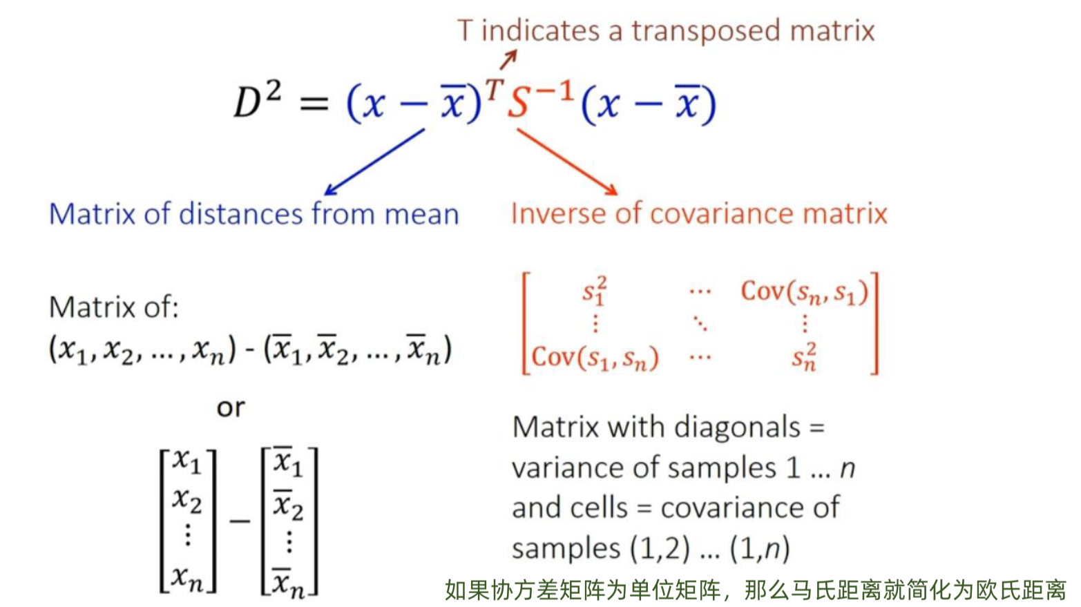
马氏距离(Mahalanobis distance) 是一种有效的计算两个向量之间相似度的方法（越小越接近样本均值也越相似，越大越远离样本均值可能是异常点），可以看作是欧氏距离的一种修正，修正了欧式距离中 各个维度（x/y/r/h）尺度不一致 且相关的问题，使得在高维空间中更具有鲁棒性

• 两个向量间的马氏距离：$D_m(x,y)=\sqrt{(x-y{)}^T{\Sigma }_{x,y}^{-1}(x-y)}$
• 其中 $\Sigma$ 是多维随机变量的 协方差矩阵，若其是单位矩阵，则马氏距离退化为欧氏距离，即各维度间独立且同分布(因为只有同分布才会方差相同，对角线是相同的方差)
• 马氏距离的平方 计算公式如下：

• 工程实践：由于协方差矩阵 S 及其逆的求解计算量比较大，我们可以将其分解为 $S=L\ast L^T$，L 为三角阵，可以使用 scipy.linalg.solve_triangular 来高效计算
  $$M^2(x,y,L{L}^T)=(x-y{)}^T(L{L}^T{)}^{-1}(x-y)=(x-y{)}^T{L}^T{L}^{-1}(x-y)=||L^{-1}(x-y)|{|}^2$$

• 代码实现如下：

def gating_distance(self, mean, covariance, measurements,
                    only_position=False, metric='maha'):
    """Compute gating distance between state distribution and measurements.
    A suitable distance threshold can be obtained from `chi2inv95`. If
    `only_position` is False, the chi-square distribution has 4 degrees of
    freedom, otherwise 2. 计算状态分布和测量值之间的门控距离
    Parameters
    ----------
    mean : ndarray
        Mean vector over the state distribution (8 dimensional).
    covariance : ndarray
        Covariance of the state distribution (8x8 dimensional).
    measurements : ndarray
        An Nx4 dimensional matrix of N measurements, each in
        format (x, y, a, h) where (x, y) is the bounding box center
        position, a the aspect ratio, and h the height.
    only_position : Optional[bool]
        If True, distance computation is done with respect to the bounding
        box center position only.
    Returns
    -------
    ndarray
        Returns an array of length N, where the i-th element contains the
        squared Mahalanobis distance between (mean, covariance) and
        `measurements[i]`.
    """
    mean, covariance = self.project(mean, covariance)
    if only_position:
        mean, covariance = mean[:2], covariance[:2, :2]
        measurements = measurements[:, :2]

    d = measurements - mean
    if metric == 'gaussian':
        return np.sum(d * d, axis=1)
    elif metric == 'maha':
        # 计算协方差矩阵的 Cholesky 分解，该分解将协方差矩阵分解为下三角矩阵 cholesky_factor，
        # 满足 covariance = cholesky_factor @ cholesky_factor.T
        cholesky_factor = np.linalg.cholesky(covariance)

        # scipy.linalg.solve_triangular 解决了一个线性方程组，形式为：cholesky_factor @ z = d.T，即求解 z = cholesky_factor^{-1} @ d.T
        z = scipy.linalg.solve_triangular(cholesky_factor, d.T, lower=True, check_finite=False, overwrite_b=True)

        # z^2 = (cholesky_factor^{-1} @ d.T)^2
        squared_maha = np.sum(z * z, axis=0)
        return squared_maha
    else:
        raise ValueError('invalid distance metric')

---

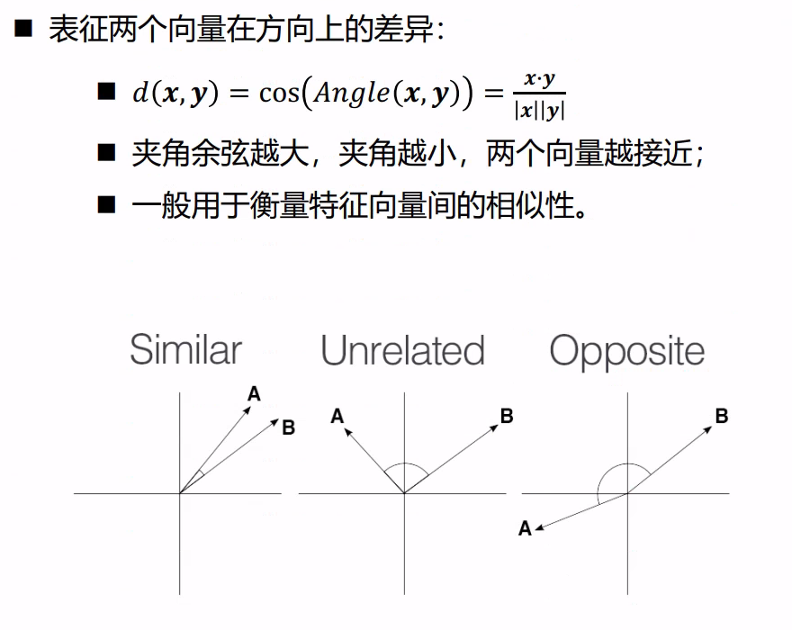
2.2、余弦距离（Cosine Distance）

• 一般用于 reid 特征间余弦距离（1 - 余弦相似度）的计算，其中 x.y 是向量 x 和向量 y 的点积，|x||y| 是向量 x 和 y 的二范数乘积
  

# 方法 1：使用 numpy 计算余弦距离
def _cosine_distance(a, b, data_is_normalized=False):
    # a和b之间的余弦距离
    # a : [NxM] b : [LxM]
    # 余弦距离 = 1 - 余弦相似度 = 1 - (a * b) / (||a|| * ||b||)
    # https://blog.csdn.net/u013749540/article/details/51813922
    """Compute pair-wise cosine distance between points in `a` and `b`.

    Parameters
    ----------
    a : array_like
        An NxM matrix of N samples of dimensionality M.
    b : array_like
        An LxM matrix of L samples of dimensionality M.
    data_is_normalized : Optional[bool]
        If True, assumes rows in a and b are unit length vectors.
        Otherwise, a and b are explicitly normalized to lenght 1.

    Returns
    -------
    ndarray
        Returns a matrix of size len(a), len(b) such that eleement (i, j)
        contains the squared distance between `a[i]` and `b[j]`.

    """
    if not data_is_normalized:
        # 需要将余弦相似度转化成类似欧氏距离的余弦距离。
        a = np.asarray(a) / np.linalg.norm(a, axis=1, keepdims=True)
        #  np.linalg.norm 操作是求向量的范式，默认是 L2 范式，等同于求向量的欧式距离。
        b = np.asarray(b) / np.linalg.norm(b, axis=1, keepdims=True)
    return 1. - np.dot(a, b.T)



# 方法 2
from scipy.spatial.distance import cosine

# 示例向量
vector_a = [1, 0, 1]
vector_b = [1, 1, 0]

# 计算余弦距离
distance = cosine(vector_a, vector_b)
print("Cosine Distance:", distance)

---

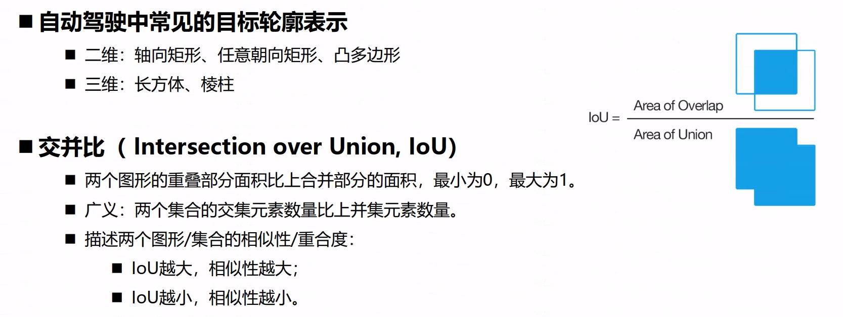
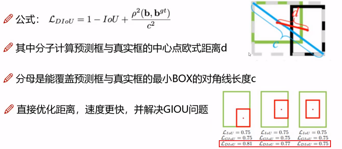
2.3、IoU 系列

• DIoU：兼顾交并比 + 预测框和真实框的中心点距离
  
• 代码实现

def iou(bbox, candidates):
    # 计算iou
    """Computer intersection over union.

    Parameters
    ----------
    bbox : ndarray(track)
        A bounding box in format `(top left x, top left y, width, height)`.
    candidates : ndarray(detections)
        A matrix of candidate bounding boxes (one per row) in the same format
        as `bbox`.

    Returns
    -------
    ndarray
        The intersection over union in [0, 1] between the `bbox` and each
        candidate. A higher score means a larger fraction of the `bbox` is
        occluded by the candidate.

    """
    bbox_tl, bbox_br = bbox[:2], bbox[:2] + bbox[2:]
    candidates_tl = candidates[:, :2]
    candidates_br = candidates[:, :2] + candidates[:, 2:]

    tl = np.c_[np.maximum(bbox_tl[0], candidates_tl[:, 0])[:, np.newaxis],
               np.maximum(bbox_tl[1], candidates_tl[:, 1])[:, np.newaxis]]
    br = np.c_[np.minimum(bbox_br[0], candidates_br[:, 0])[:, np.newaxis],
               np.minimum(bbox_br[1], candidates_br[:, 1])[:, np.newaxis]]
    wh = np.maximum(0., br - tl)

    area_intersection = wh.prod(axis=1)
    area_bbox = bbox[2:].prod()
    area_candidates = candidates[:, 2:].prod(axis=1)
    return area_intersection / (area_bbox + area_candidates - area_intersection)


def iou_cost(tracks, detections, track_indices=None, detection_indices=None):
    # 计算 track 和 detection 之间的 iou 距离矩阵
    """An intersection over union distance metric.

    Parameters
    ----------
    tracks : List[deep_sort.track.Track]
        A list of tracks.
    detections : List[deep_sort.detection.Detection]
        A list of detections.
    track_indices : Optional[List[int]]
        A list of indices to tracks that should be matched. Defaults to
        all `tracks`.
    detection_indices : Optional[List[int]]
        A list of indices to detections that should be matched. Defaults
        to all `detections`.

    Returns
    -------
    ndarray
        Returns a cost matrix of shape
        len(track_indices), len(detection_indices) where entry (i, j) is
        `1 - iou(tracks[track_indices[i]], detections[detection_indices[j]])`.

    """
    if track_indices is None:
        track_indices = np.arange(len(tracks))
    if detection_indices is None:
        detection_indices = np.arange(len(detections))

    cost_matrix = np.zeros((len(track_indices), len(detection_indices)))
    for row, track_idx in enumerate(track_indices):
        # 丢失超过 1 帧的 track，直接设置为最大代价（TODO: 为什么是 INFTY_COST？为什么丢失超过 1 帧的 track 会直接设置为最大代价？可以考虑放开限制，增加被遮挡找回的可能性）
        # 如果丢失超过 1 帧的 track，直接设置为最大代价，这样在后续的匹配过程中，这个 track 不会被匹配到任何 detection。
        # 如果一个目标丢失太久（超过 1 帧），它可能已经不再出现在场景中，因此被认为不再是一个有效的轨迹
        # 如果一个目标被短暂遮挡丢失并且之后重新出现，那么设置丢失超过 1 帧的轨迹为最大代价（INFTY_COST）的策略可能会错过这个目标。
        # 这种情况下，目标可能并没有真正消失，而是因为某种原因（比如遮挡）短暂未被跟踪到
        if tracks[track_idx].time_since_update > 1:
            cost_matrix[row, :] = linear_assignment.INFTY_COST
            continue

        bbox = tracks[track_idx].to_tlwh()
        candidates = np.asarray([detections[i].tlwh for i in detection_indices])
        cost_matrix[row, :] = 1. - iou(bbox, candidates)

    return cost_matrix

---

三、最优关联匹配：匈牙利匹配

• 如何定义最优的关联匹配？
  • 直觉思维：让最接近/相似的目标匹配上（最近邻匹配）
  • 大局观：让匹配相似度的总和最大（匈牙利匹配）
  • 不做选择：每一种可能我都要（概率数据关联/多假设跟踪）
• 这里我们主要介绍匈牙利匹配

3.1、二分图的定义及其在跟踪中的理解

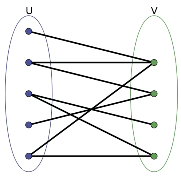
• 二分图的定义：二分图是能分成两组（假设是 U 和 V），其中 U 上的点不能相互连通，只能连去 V 中的点；V 中的点也不能相互连通，只能连去 U 中的点
• 二分图在跟踪中的理解：可以把二分图理解为视频中连续两帧中的所有检测框，第一帧所有检测框的集合称为 U，第二帧所有检测框的集合称为 V，同一帧的不同检测框不会为同一个目标，所以不需要互相关联，相邻两帧的检测框需要相互联通，最终将相邻两帧的检测框尽量完美地两两匹配起来

3.2、匈牙利算法、KM 算法

• 匈牙利算法定义及缺点：

  • 定义： 是一种在多项式时间内求解任务分配问题的组合优化算法，在多目标跟踪问题中可以简单理解为寻找 前后两帧的若干目标的匹配最优解 的一种算法
  • 缺点： 将每个匹配对象的地位视为相同，在这个前提下求解最大匹配，这个和我们研究的多目标跟踪问题有些不合，因为每个匹配对象不可能是同等地位的，总有一个真实目标是我们要找的最佳匹配，而这个真实目标应该拥有更高的权重，在此基础上匹配的结果才能更贴近真实情况

• KM 算法形象的解释

  • KM 算法定义和优点：

    • 定义：解决的是带权二分图的最优匹配问题，给每条连接关系加入了权重（权重的计算可通过前后两帧状态变量的马氏距离 或者 reid 特征的余弦相似度 或者 状态变量间的IoU 等）
    • 优点：可以实现最优匹配，而不是简单的取相似度最大的进行匹配

  • KM 算法匹配原则：

    • 首先，初始化各个顶点（称为顶标），将左边的顶点赋值为与其相连边的最大权重（权重的计算可通过前后两帧状态变量的马氏距离 或者 reid 特征的余弦相似度 或者 状态变量间的IoU 等），右边的顶点赋值为 0
    • 然后，只和权重与左边分数（顶标）相同的边进行匹配
    • 最后，若找不到边匹配，对此条路径 所有冲突边的顶点做加减操作，令左边顶点值减 d，右边顶点值加 d（参数 d 这里取 0.1）

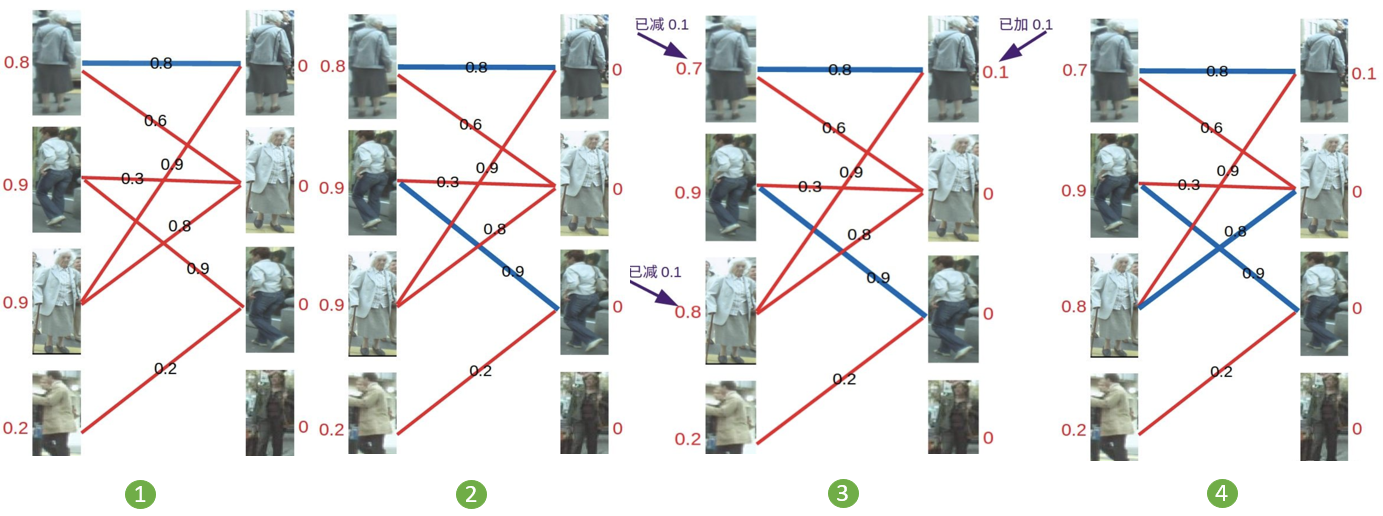
  • KM 算法匹配示例：

    • 第 1 步： 对于左 1，与顶标分值相同的边标蓝
    • 第 2 步： 对于左 2，与顶标分值相同的边标蓝
    • 第 3 步： 对于左 3，发现与右 1 已经与左 1 配对，而此时左 3 和 左 1 都无法更换匹配的边（找不到其它权值大于等于左顶标加右顶标的边），此时根据 KM 算法匹配原则，应对所有冲突的边的顶点做加减操作，令左边顶点值减 0.1，右边顶点值加 0.1
    • 第 4 步： 进行加减操作后再进行匹配，发现左3 多了一条可匹配的边（左 3 对右 2 的匹配要求只需权重大于等于 0.8+0），所以左 3 与右 2 匹配
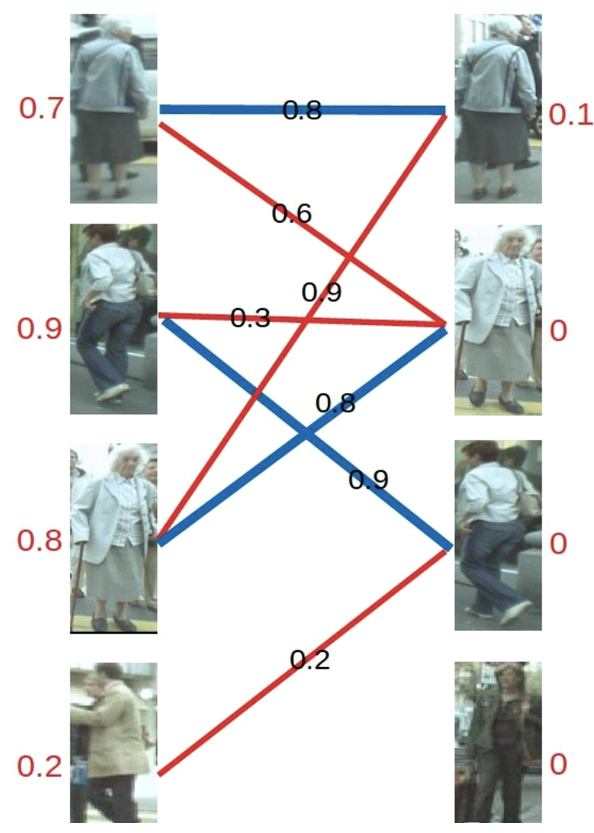
    • 第 5 步： 对于左 4，由于左 4 唯一的匹配对象右 3 已被左 2 匹配，发生冲突，进行一轮加减操作再进行匹配，左四还是匹配失败，两轮以后左 4 期望值降为 0，放弃匹配左 4
      

3.3、匈牙利算法的实现

linear_sum_assignment 求的是最大匹配，使得代价最小，传入的是 cost 距离矩阵（iou 距离或 cos 距离+马氏距离限制）

import numpy as np
from scipy.optimize import linear_sum_assignment

# 代价矩阵 4*4， 前后帧都有四个目标：权重可通过马氏距离或者余弦相似度计算
cost = np.array([[0.8, 0.6, 0, 0],
                 [0, 0.3, 0.9, 0],
                 [0.9, 0.8, 0, 0],
                 [0, 0, 0.2, 0]])

# 匹配结果：该方法的目的是代价最小，这里是求最大匹配，所以将 cost 取负数
row_ind, col_ind = linear_sum_assignment(-cost)

# 对应的行索引
print("行索引：\n{}".format(row_ind))

# 对应行索引的最优指派的列索引
print("列索引：\n{}".format(col_ind))

# 提取每个行索引的最优指派列索引所在的元素，形成数组
print("匹配度：\n{}".format(cost[row_ind, col_ind]))


# 输出结果如下
行索引：
[0 1 2 3]
列索引：
[0 2 1 3]
匹配度：
[0.8 0.9 0.8 0. ]  # 匹配度为 0，说明没有匹配上