


文章目录
本课程来自深度之眼deepshare.net,部分截图来自课程视频。
内容简介
今天学习pytorch中剩下的14种损失函数;学习优化器optimizer的基本属性、基本方法和作用。
本节第二部分学习优化器的基本概念,了解pytorch中optimizer的基本属性和方法
http://pytorch.org/docs/master/nn.html
损失函数
继续上一节的内容,继续学习剩下的14中损失函数:
5.nn.L1Loss
6.nn.MSELoss
7.nn.SmoothL1Loss
8.nn.PoissonNLLLoss
9.nn.KLDivLoss
10.nn.MarginRankingLoss
11.nn.MultiLabelMarginLoss
12.nn.SoftMarginLoss
13.nn.MultilabelSoftMarginLoss
14.nn.MultiMarginLoss
15.nn.TripletMarginLoss
16.nn.HingeEmbeddingLoss
17.nn.CosineEmbeddingLoss
18.nn.CTCLoss
5.nn.L1Loss&6.nn.MSELoss
5、nn.L1Loss
功能:计算inputs与target之差的绝对值:
l
n
=
∣
x
n
−
y
n
∣
l_n=|x_n-y_n|
ln=∣xn−yn∣
6、nn.MSELoss
功能:计算inputs与target之差的平方:
l
n
=
(
x
n
−
y
n
)
2
l_n=(x_n-y_n)^2
ln=(xn−yn)2
两个损失函数的主要参数:
·reduction:计算模式,可为none/sum/mean
这个参数和之前讲过的一样,none就是不对loss进行处理
sum是对所有loss求和
mean是对所有loss求平均
后面所有函数都一样的,不在赘述。
none-逐个元素计算
sum-所有元素求和,返回标量
mean-加权平均,返回标量
7、SmoothLlLoss
功能:平滑的L1Loss
l
o
s
s
(
x
,
y
)
=
1
n
∑
i
z
i
loss(x,y)=\frac{1}{n}\sum_iz_i
loss(x,y)=n1i∑zi
其中:
z
i
=
{
0.5
(
x
i
−
y
i
)
2
,
i
f
∣
x
i
−
y
i
∣
<
1
∣
x
i
−
y
i
∣
−
0.5
,
o
t
h
e
r
w
i
s
e
z_i=\left\{\begin{matrix} 0.5(x_i-y_i)^2, \space if|x_i-y_i|<1\\ |x_i-y_i|-0.5,\space otherwise \end{matrix}\right.
zi={0.5(xi−yi)2, if∣xi−yi∣<1∣xi−yi∣−0.5, otherwise
主要参数:
·reduction:计算模式,可为none/sum/mean
none-逐个元素计算
sum-所有元素求和,返回标量
mean-加权平均,返回标量
从图像中可以看到在-1至1之间,是一个平滑的曲线,其他地方要比L1loss要小0.5

8、PoissonNLLLoss
功能:泊松分布的负对数似然损失函数
主要参数:
·log input:输入是否为对数形式,决定计算公式
·full:计算所有loss,默认为Falseo
·eps:修正项,避免log(input)为nan,默认值为一个很小的数字:1e-08
计算公式:
loginput=True:
loss(input,target)=exp(input)-target * input
log_input=False:
loss(input,target)=input-target* log(input+eps)
9、nn.KLDivLoss
功能:计算KLD(divergence),KL散度,就是相对熵,用来衡量两个分布之间的相似性(距离)。
数学上的计算公式如下:
D
K
L
(
P
∣
∣
Q
)
=
E
x
∼
p
[
l
o
g
P
(
x
)
Q
(
x
)
]
=
E
x
∼
p
[
l
o
g
P
(
x
)
−
l
o
g
Q
(
x
)
]
=
∑
i
=
1
N
P
(
x
i
)
(
l
o
g
P
(
x
i
)
−
l
o
g
Q
(
x
i
)
)
D_{KL}(P||Q)=E_{x\sim p}\left [log\frac{P(x)}{Q(x)}\right ]=E_{x\sim p}[logP(x)-logQ(x)]=\sum_{i=1}^NP(x_i)\left(logP(x_i)-logQ(x_i)\right)
DKL(P∣∣Q)=Ex∼p[logQ(x)P(x)]=Ex∼p[logP(x)−logQ(x)]=i=1∑NP(xi)(logP(xi)−logQ(xi))
PyTorch中的计算公式如下:
l
n
=
y
n
⋅
(
l
o
g
y
n
−
x
n
)
l_n=y_n\cdot(logy_n-x_n)
ln=yn⋅(logyn−xn)
由于是对一个样本进行计算,所以PyTorch中的计算公式没有求和符号,第一项
y
n
y_n
yn就是数据集中的标签,对应的是
P
(
x
i
)
P(x_i)
P(xi),然后括号里面的第一项
l
o
g
y
n
logy_n
logyn和
l
o
g
P
(
x
i
)
logP(x_i)
logP(xi)也是对应的。但是最后一项不一样,PyTorch中只减去输入的数据
x
n
x_n
xn,因此,要手工对这个东西提前进行处理,使得这一项和数学中的计算公式一样,也就是要计算一个概率然后求log,也就是我们的注意事项中的内容:
注意事项:需提前将输入计算log-probabilities,如通过nn.logsoftmax()
主要参数:
·reduction:none/sum/mean/batchmean
batchmean-batchsize维度求平均值(特殊)
none-逐个元素计算
sum-所有元素求和,返回标量
mean-加权平均,返回标量
10、nn.MarginRankingLoss
功能:计算两个向量之间的相似度,用于排序任务
l
o
s
s
(
x
,
y
)
=
m
a
x
(
0
,
−
y
∗
(
x
1
−
x
2
)
+
m
a
r
g
i
n
)
loss(x,y)=max(0,-y*(x1-x2)+margin)
loss(x,y)=max(0,−y∗(x1−x2)+margin)
y=1时,希望x1比x2大,当x1>x2时,不产生loss
y=-1时,希望x2比x1大,当x2>x1时,不产生loss
特别说明:该方法计算两组数据之间的差异,返回一个n*n的loss 矩阵
主要参数:
·margin:边界值,x1与x2之间的差异值,默认为0
·reduction:计算模式,可为none/sum/mean
x1=torch.tensor([[1],[2],[3]],dtype=torch.float)
x2=torch.tensor([[2],[2],[2]],dtype=torch.float)
target=torch.tensor([1,1,-1],dtype=torch.float)
loss_f_none=nn.MarginRankingLoss(margin=e,reduction='none')
loss=loss_f_none(x1,x2,target)
结果:
由于输入张量大小是3,则loss是3*3的大小
看一下第一行的110如何得来:用x1的第一个元素:1和x2的三个元素[2],[2],[2]]进行比较,我们希望得到结果是target:[1,1,-1]:
先看第一个比较,由于target=1,希望x1比x2大,但是实际上x1比x2小,因此产生了loss=1
再看第二个比较,由于target=1,希望x1比x2大,但是实际上x1比x2小,因此产生了loss=1
再看第三个比较,由于target=-1,希望x2比x1大,实际上x2比x1大,因此loss=0
11、nn.MultiLabelMarginLoss
功能:多标签边界损失函数,例如,多标签是指一张图片对应多个类别,不是多分类,多分类是一个图片属于一个类别,但是有多个类别。
例如下图对应云、树,海,草地多个标签:

l
o
s
s
(
x
,
y
)
=
∑
i
j
m
a
x
(
0
,
1
−
(
x
[
y
[
j
]
]
−
x
[
i
]
)
)
x
.
s
i
z
e
(
0
)
loss(x,y)=\sum_{ij}\frac{max(0,1-(x[y[j]]-x[i]))}{x.size(0)}
loss(x,y)=ij∑x.size(0)max(0,1−(x[y[j]]−x[i]))
w
h
e
r
e
i
=
=
0
t
o
x
.
s
i
z
e
(
0
)
,
j
=
=
0
t
o
y
.
s
i
z
e
(
0
)
,
y
[
j
]
≥
0
,
a
n
d
i
<
>
y
[
j
]
f
o
r
a
l
l
i
a
n
d
j
where \space i==0\space to \space x.size(0),j==0\space to \space y.size(0),y[j]≥0,and\space i<>y[j] \space for \space all \space i \space and \space j
where i==0 to x.size(0),j==0 to y.size(0),y[j]≥0,and i<>y[j] for all i and j
分母是神经元的个数,分子是用标签的神经元减去非标签的神经元
举例:四分类任务,样本x属于0类和3类,

四个神经元,对应的输出是第零个和第三个神经元,则减去的x[i]是中间两个。也就是说第0号神经元要比第1号和第2号神经元的和要大,且大过1,否则就会产生loss,也就是说训练的目的就是要让0号神经元的输出尽可能的大。
样本x属于0类和3类的标签是[0,3,-1,-1],不是[1,0,0,1 ]
主要参数:
·reduction:计算模式,可为none/sum/mean
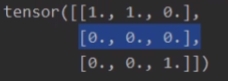
x=torch.tensor([[0.1,0.2,0.4,0.8]])
y=torch.tensor([[0,3,-1,-1]],dtype=torch.1ong)
loss_f=nn.MultilabelMarginLoss(reduction='none')
loss=1oss_f(x,y)
print(1oss)
结果是:0.85
计算方式是:
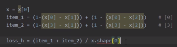
其中item_1是对应第0个神经元减去不是分类的1和2号神经元:(1-(0.1-0.2))+(1-(0.1-0.4))=1.3
item_2是对应第3个神经元减去不是分类的1和2号神经元:(1-(0.8-0.2))+(1-(0.8-0.4))=0.6
x.shape是4(总共有四个神经元)
12、nn.SoftMarginLoss
功能:计算二分类的logistic损失
l
o
s
s
(
x
,
y
)
=
∑
i
l
o
g
(
1
+
e
x
p
(
−
y
[
i
]
∗
x
[
i
]
)
)
x
.
n
e
l
e
m
e
n
t
(
)
loss(x,y)=\sum_i\frac{log(1+exp(-y[i]*x[i]))}{x.nelement()}
loss(x,y)=i∑x.nelement()log(1+exp(−y[i]∗x[i]))
主要参数:
·reduction:计算模式,可为none/sum/mean
13、nn.MultiLabelSoftMarginLoss
功能:SoftMarginLoss多标签版本
l
o
s
s
(
x
,
y
)
=
−
1
C
∗
∑
i
y
[
i
]
∗
l
o
g
(
(
1
+
e
x
p
(
−
x
[
i
]
)
)
−
1
)
+
(
1
−
y
[
i
]
)
∗
l
o
g
(
e
x
p
(
−
x
[
i
]
)
1
+
e
x
p
(
−
x
[
i
]
)
)
loss(x,y)=-\frac{1}{C}*\sum_iy[i]*log((1+exp(-x[i]))^{-1})+(1-y[i])*log(\frac{exp(-x[i])}{1+exp(-x[i])})
loss(x,y)=−C1∗i∑y[i]∗log((1+exp(−x[i]))−1)+(1−y[i])∗log(1+exp(−x[i])exp(−x[i]))
i是第i个神经元,C是标签的数量,当y=1时用前面部分计算loss,否则用后面部分计算loss
主要参数:
·weight:各类别的loss设置权值
·reduction:计算模式,可为none/sum/mean
14、nn.MultiMarginLoss
功能:计算多分类的折页损失
l
o
s
s
(
x
,
y
)
=
∑
i
m
a
x
(
0
,
(
m
a
r
g
i
n
−
x
[
y
]
+
x
[
i
]
)
)
p
x
.
s
i
z
e
(
0
)
loss(x,y)=\frac{\sum_imax(0,(margin-x[y]+x[i]))^p}{x.size(0)}
loss(x,y)=x.size(0)∑imax(0,(margin−x[y]+x[i]))p
还可以为各个类别设置不同权值:
l
o
s
s
(
x
,
y
)
=
∑
i
m
a
x
(
0
,
w
[
y
]
∗
(
m
a
r
g
i
n
−
x
[
y
]
+
x
[
i
]
)
)
p
x
.
s
i
z
e
(
0
)
loss(x,y)=\frac{\sum_imax(0,w[y]*(margin-x[y]+x[i]))^p}{x.size(0)}
loss(x,y)=x.size(0)∑imax(0,w[y]∗(margin−x[y]+x[i]))p
其中,0≤y≤x.size(1) ; i == 0 to x.size(0) and i≠y; p==1 or p ==2; w[y]为各类别的weight。
主要参数:
·p:可选1或2,默认值为1
·weight:各类别的loss设置权值
·margin:边界值
·reduction:计算模式,可为none/sum/mean
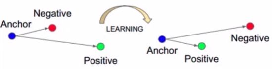
15、nn.TripletMarginLoss
功能:计算三元组损失,人脸验证中常用(自己的脸和自己脸要近一点,和别人的脸要远一点)
通过学习使得positive和anchor的距离要比negative和anchor的距离要小,否则会产生loss,距离计算一般采用L2 norm
L
(
a
,
p
,
n
)
=
m
a
x
{
d
(
a
i
,
p
i
)
−
d
(
a
i
,
n
i
)
+
m
a
r
g
i
n
,
0
}
L(a,p,n)=max\{d(a_i,p_i)-d(a_i,n_i)+margin,0\}
L(a,p,n)=max{d(ai,pi)−d(ai,ni)+margin,0}
d
(
x
i
,
y
i
)
=
∣
∣
x
i
−
y
i
∣
∣
p
d(x_i,y_i)=||x_i-y_i||_p
d(xi,yi)=∣∣xi−yi∣∣p
主要参数:
·p:范数的阶,默认为2
·margin:边界值
·reduction:计算模式,可为none/sum/mean
16、nn.HingeEmbeddingLoss
功能:计算两个输入的相似性,常用于非线性embedding和半监督学习
l
n
=
{
x
n
,
i
f
y
n
=
1
m
a
x
{
0
,
Δ
−
x
n
}
,
i
f
y
n
=
−
1
l_n=\left\{\begin{matrix} x_n,\space if \space y_n=1\\ max\{0,\Delta-x_n\},\space if\space y_n=-1 \end{matrix}\right.
ln={xn, if yn=1max{0,Δ−xn}, if yn=−1
特别注意:输入x应为两个输入之差的绝对值
主要参数:
·margin:边界值
·reduction:计算模式,可为none/sum/mean
17、nn.CosineEmbeddingLoss
功能:采用余弦相似度计算两个输入的相似性
l
o
s
s
(
x
,
y
)
=
{
1
−
c
o
s
(
x
1
,
x
2
)
,
i
f
y
=
1
m
a
x
{
0
,
c
o
s
(
x
1
,
x
2
)
−
m
a
r
g
i
n
}
,
i
f
y
=
−
1
loss(x,y)=\left\{\begin{matrix} 1-cos(x_1,x_2),\space if \space y=1\\ max\{0,cos(x_1,x_2)-margin\},\space if\space y=-1 \end{matrix}\right.
loss(x,y)={1−cos(x1,x2), if y=1max{0,cos(x1,x2)−margin}, if y=−1
cos主要是计算x1和x2在方向上的差异,不是大小差异
c
o
s
(
θ
)
=
A
⋅
B
∣
∣
A
∣
∣
∣
∣
B
∣
∣
=
∑
i
=
1
n
A
i
×
B
i
∑
i
=
1
n
(
A
i
)
2
×
∑
i
=
1
n
(
B
i
)
2
cos(\theta)=\frac{A\cdot B}{||A||||B||}=\frac{\sum_{i=1}^nA_i×B_i}{\sqrt{\sum_{i=1}^n(A_i)^2}×\sqrt{\sum_{i=1}^n(B_i)^2}}
cos(θ)=∣∣A∣∣∣∣B∣∣A⋅B=∑i=1n(Ai)2×∑i=1n(Bi)2∑i=1nAi×Bi
主要参数:
·margin:可取值[-1,1](因为cos的值域也是这个),推荐为[0,0.5]
·reduction:计算模式,可为none/sum/mean
18、nn.CTCLoss
功能:计算CTC损失,解决时序类数据的分类Connectionist Temporal Classification,公式参考参考文献。
主要参数:
·blank:blank label
·zero infinity:无穷大的值或梯度置0
·reduction:计算模式,可为none/sum/mean
参考文献:
A.Graves et al.:Connectionist Temporal Classification:Labelling Unsegmented Sequence Data with Recurrent Neural Networks
优化器 Optimizer
什么是优化器
pytorch的优化器:管理并更新模型中可学习参数的值,使得模型输出更接近真实标签
下面讲解梯度相关概念:
导数:函数在指定坐标轴上的变化率
方向导数:指定方向上的变化率
梯度:一个向量,方向为方向导数取得最大值的方向,大小是变化率
optimizer的属性
基本属性
·defaults:优化器超参数
·state:参数的缓存,如momentum的缓存
·param_groups:管理的参数组是一个list每一个元素是一个字典,有很多key-value对。
·_step_count:记录更新次数,学习率调整中使用
optimizer的方法
·zero_grad():清空所管理参数的梯度
pytorch特性:张量梯度不自动清零
·step():执行一步更新
·add_param_group():添加参数组,当要分段训练的时候就要为每个分段分别定义参数组
模型训练状态的保存和加载:
·state_dict():获取优化器当前状态信息字典
·load_state_dict():加载状态信息字典


 276
276


 被折叠的 条评论
为什么被折叠?
被折叠的 条评论
为什么被折叠?
 到【灌水乐园】发言


