


本文内容整理自深度之眼《GNN核心能力培养计划》
创建简单数据集
创建自己的数据集,并用于节点分类、边预测以及图分类任务。
自定义数据集要继承DGLDataset这个类,并实现三个方法(其实和Torch的Dataset非常像)
__getitem__(self, i): retrieve the i-th example of the dataset. An example often contains a single DGL graph, and occasionally its label. 获取第i个图对象,如果有ground truth,也一并获取到。
__len__(self): the number of examples in the dataset. 读取到的对象个数
process(self): load and process raw data from disk.
本节仍然用karate数据集,不过这次我们自己来创建图,不是直接用DGL自带的:
Zachary’s karate club is a social network of a university karate club, described in the paper “An Information Flow Model for Conflict and Fission in Small Groups” by Wayne W. Zachary. The network became a popular example of community structure in networks after its use by Michelle Girvan and Mark Newman in 2002. Official website:
原始数据准备
先下载原始数据到本地:
import urllib.request
import pandas as pd
urllib.request.urlretrieve('https://data.dgl.ai/tutorial/dataset/members.csv', './members.csv')
urllib.request.urlretrieve('https://data.dgl.ai/tutorial/dataset/interactions.csv', './interactions.csv')
当前文件夹下面会有:

然后用pandas读一把,并显示前几行
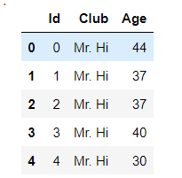
members = pd.read_csv('./members.csv')
members.head()
第二列应该是俱乐部的名称,还有一个名称叫:Officer
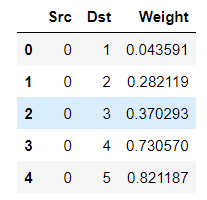
interactions = pd.read_csv('./interactions.csv')
interactions.head()
这里是邻接表,最后一列是权重
原始数据中,我们用members中的id做节点,interactions的src和dst做边,members的age做节点特征,interactions的Weight做边的特征。members的Club做label。
建图
具体看注释
import dgl
from dgl.data import DGLDataset
import torch
import os

#继承DGLDataset类创建自己的数据集类
class KarateClubDataset(DGLDataset):
    def __init__(self):
        super().__init__(name='karate_club')

    def process(self):
        # 读取csv文件得到DataFrame
        nodes_data = pd.read_csv('./members.csv')
        edges_data = pd.read_csv('./interactions.csv')

        # DataFrame里面切出特征列,对于标签列['Club']这里做了独热编码转化
        node_features = torch.from_numpy(nodes_data['Age'].to_numpy())
        node_labels = torch.from_numpy(nodes_data['Club'].astype('category').cat.codes.to_numpy())
        edge_features = torch.from_numpy(edges_data['Weight'].to_numpy())

        # 读节点
        edges_src = torch.from_numpy(edges_data['Src'].to_numpy())
        edges_dst = torch.from_numpy(edges_data['Dst'].to_numpy())

        # 创建图,最后一个参数是节点数量
        self.graph = dgl.graph((edges_src, edges_dst), num_nodes=nodes_data.shape[0])
        self.graph.ndata['feat'] = node_features
        self.graph.ndata['label'] = node_labels
        self.graph.edata['weight'] = edge_features

        # If your dataset is a node classification dataset, you will need to assign
        # masks indicating whether a node belongs to training, validation, and test set.
        # 划分训练、验证、测试集
        n_nodes = nodes_data.shape[0]
        n_train = int(n_nodes * 0.6)
        n_val = int(n_nodes * 0.2)
        train_mask = torch.zeros(n_nodes, dtype=torch.bool)
        val_mask = torch.zeros(n_nodes, dtype=torch.bool)
        test_mask = torch.zeros(n_nodes, dtype=torch.bool)

        # 划分的工具就是mask
        train_mask[:n_train] = True
        val_mask[n_train:n_train + n_val] = True
        test_mask[n_train + n_val:] = True
        self.graph.ndata['train_mask'] = train_mask
        self.graph.ndata['val_mask'] = val_mask
        self.graph.ndata['test_mask'] = test_mask

    def __getitem__(self, i):
        return self.graph

    def __len__(self):
        return 1#这里只有一个图

dataset = KarateClubDataset()
graph = dataset[0]

print(graph)
结果:

创建图分类数据集
要做图分类,那么图应该有很多个,上面的例子只有一个图。__getitem__也只会得到一个结果。
准备数据
两个原始文件的信息如下所示:
graph_edges.csv: containing three columns:
graph_id: the ID of the graph.src: the source node of an edge of the given graph.dst: the destination node of an edge of the given graph.
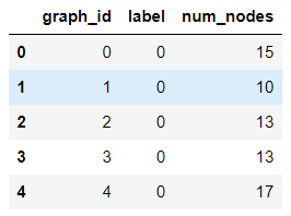
graph_properties.csv: containing three columns:
graph_id: the ID of the graph.label: the label of the graph.num_nodes: the number of nodes in the graph.
下载到本地后读取看看什么样:
urllib.request.urlretrieve(
    'https://data.dgl.ai/tutorial/dataset/graph_edges.csv', './graph_edges.csv')
urllib.request.urlretrieve(
    'https://data.dgl.ai/tutorial/dataset/graph_properties.csv', './graph_properties.csv')
edges = pd.read_csv('./graph_edges.csv')
properties = pd.read_csv('./graph_properties.csv')
打印信息看看:
edges.head()
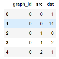
上面的graph_id是不同图的编号,这里只显示了0号。
properties.head()
建图
#继承DGLDataset定义自己的数据集
class SyntheticDataset(DGLDataset):
def __init__(self):
super().__init__(name='synthetic')
def process(self):
# 读本地文件到DF
edges = pd.read_csv('./graph_edges.csv')
properties = pd.read_csv('./graph_properties.csv')
self.graphs = []#图列表
self.labels = []#图标签列表
# Create a graph for each graph ID from the edges table.
# First process the properties table into two dictionaries with graph IDs as keys.
# The label and number of nodes are values.
label_dict = {}# 保存图的label,就是properties中的第二列
num_nodes_dict = {}#保存图的节点数,就是properties中的第三列
for _, row in properties.iterrows():# 遍历DF的每一行,将properties信息读取到字典中
label_dict[row['graph_id']] = row['label']
num_nodes_dict[row['graph_id']] = row['num_nodes']
# For the edges, first group the table by graph IDs.
# 这里将edges中的边信息按图进行分组,就是具有相同图graph_id的边会分在一组
edges_group = edges.groupby('graph_id')
# For each graph ID...
# 对每个graph_id(也就是每个图,不同id不同的图)都分别读取点边,然后建图
for graph_id in edges_group.groups:
# Find the edges as well as the number of nodes and its label.
edges_of_id = edges_group.get_group(graph_id)
src = edges_of_id['src'].to_numpy()#读点
dst = edges_of_id['dst'].to_numpy()
num_nodes = num_nodes_dict[graph_id]#取节点个数作为建图的第三个参数
label = label_dict[graph_id]#取标签
# Create a graph and add it to the list of graphs and labels.
g = dgl.graph((src, dst), num_nodes=num_nodes)
self.graphs.append(g)
self.labels.append(label)
# Convert the label list to tensor for saving.
self.labels = torch.LongTensor(self.labels)
def __getitem__(self, i):
return self.graphs[i], self.labels[i]
def __len__(self):
return len(self.graphs)
dataset = SyntheticDataset()
graph, label = dataset[0]#打印0号图
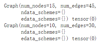
print(graph, label)
graph, label = dataset[1]#打印1号图
print(graph, label)
大图的处理:Sampling
理论
这个知识点来自:这一篇综述
Graph neural networks: A review of methods and applications
里面有些idea可以深入:
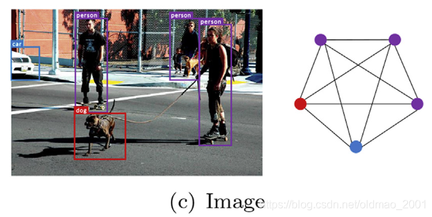
CV的bounding box可以建图,并分析里面的物体的关系:
先说下为什么会需要采样,因为在一些图上,一个节点的邻居如果是
1
0
4
10^4
104个,那么考虑两层邻居,就需要考虑
1
0
4
×
1
0
4
10^4\times10^4
104×104个结点,计算量是指数级增长的,因此我们通常是使用一个固定大小的窗口对节点进行采样。
对应原文3.4节:
GNN models aggregate messages for each node from its neighborhoodin the previous layer. Intuitively, if we track back multiple GNN layers,the size of supporting neighbors will grow exponentially with the depth.
3.4.1 Node sampling
通常窗口大小为:2到50。(GraphSAGE论文观点)
或者通过邻居的重要程度来进行采样。(PinSage论文)
3.4.2 Layer sampling
通过控制每一层邻居数量来减少计算量。(FastGCN)
3.4.3 Subgraph sampling
这个思想是由于随机采样不能考虑所有类型节点,因此在采样时考虑将所有邻居进行聚类分子图,再从结果中分别采样。
实操
然后看实例,来自官网。
DGL上将大图采样节点的方法称为message flow graphs (MFG),整个MFG的思路,做法对应起来,也可以这样想,采样后相当于我们把原图求了个子图,然后再进行GCN操作。
下面根据官网的例子来看下代码,使用的数据集的斯坦福提供的OGB的大图( 170 thousand nodes and 1 million edges)
环境准备和数据载入
跑之前先装ogb的包
pip install ogb
清华源秒好
import dgl
import torch
import numpy as np
from ogb.nodeproppred import DglNodePropPredDataset

dataset = DglNodePropPredDataset('ogbn-arxiv')

device = ''
if torch.cuda.is_available():
    device = 'cuda:0'
else:
    device = 'cpu'
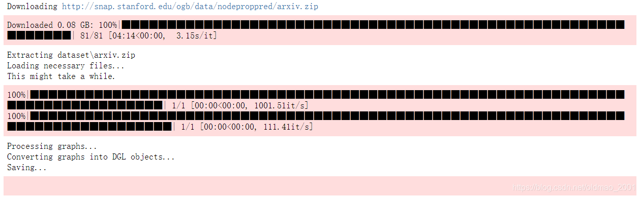
第一次跑要下载数据

搞定
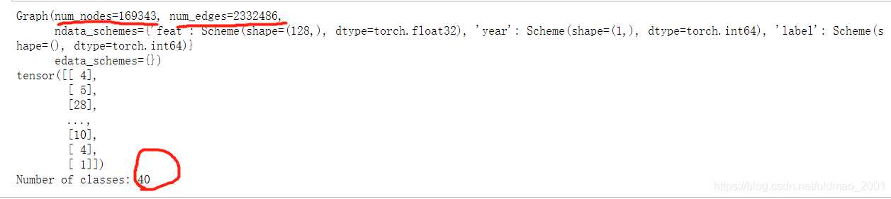
打印信息,这个数据集只包含一个图
graph, node_labels = dataset[0]
# Add reverse edges since ogbn-arxiv is unidirectional.
graph = dgl.add_reverse_edges(graph)
graph.ndata['label'] = node_labels[:, 0]
print(graph)
print(node_labels)

node_features = graph.ndata['feat']
num_features = node_features.shape[1]
num_classes = (node_labels.max() + 1).item()
print('Number of classes:', num_classes)
获取划分好的训练验证测试集
idx_split = dataset.get_idx_split()
train_nids = idx_split['train']
valid_nids = idx_split['valid']
test_nids = idx_split['test']
采样
先要定义dgl.dataloading.MultiLayerNeighborSampler,这里要指定固定大小的邻居窗口
然后作为参数传入:dgl.dataloading.NodeDataLoader
# 有两层,每层每个节点采样4个邻居
sampler = dgl.dataloading.MultiLayerNeighborSampler([4, 4])
train_dataloader = dgl.dataloading.NodeDataLoader(
    # The following arguments are specific to NodeDataLoader.
    graph,              # The graph
    train_nids,         # The node IDs to iterate over in minibatches
    sampler,            # The neighbor sampler
    device=device,      # Put the sampled MFGs on CPU or GPU
    # The following arguments are inherited from PyTorch DataLoader.
    batch_size=1024,    # Batch size
    shuffle=True,       # Whether to shuffle the nodes for every epoch
    drop_last=False,    # Whether to drop the last incomplete batch
    num_workers=0       # Number of sampler processes
)
试着把batch信息和输入输出节点打印一下,这里的input_nodes, output_nodes前面几个id为什么是一样的?可以思考一下,后面MFG讲解有答案。
input_nodes, output_nodes, mfgs = example_minibatch = next(iter(train_dataloader))
print(example_minibatch)
print("To compute {} nodes' outputs, we need {} nodes' input features".format(len(output_nodes), len(input_nodes)))

这里每个batch是1024个结点,如果是完全图的话,那么输入的节点理论上是1024×4×4=16384个,但是这里是12696,说明缺一些边。
这里是最简单的情况,还可以有自定义的sampler,异质图的sampler,自定义的异质图sampler。
根据上面打印信息我们可以看到NodeDataLoader包含三个东西:
1.An ID tensor for the input nodes, i.e., nodes whose input features are needed on the first GNN layer for this minibatch.输入节点的ID
2.An ID tensor for the output nodes, i.e. nodes whose representations are to be computed.输出节点的ID,可以是中间层,也可能是最后的输出层
3.A list of MFGs storing the computation dependencies for each GNN layer.每层的消息传递关系
MFG就是每一层里面从那几个节点(经过采样后)进行消息汇聚到当前节点的关系。原文有动图,我还是重新截图写下吧。
MFG
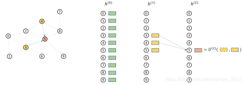
这个例子演示sample size为2的情况。
第一步,以节点5为例来计算,常规要算他的所有邻居,再包含他本身,共有234689+5共7个节点

但是我们sample size为2,因此从邻居节点随机采样2个节点,变成:34+5
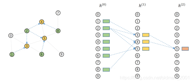
再来看34+5三个节点的前一层(跳)邻居
3节点对应01256+3
4节点对应258+4
5节点对应234689+5

再次每个节点采样2个邻居:
3节点对应12+3
4节点对应28+4
5节点对应26+5
去掉没有采样的节点变成:
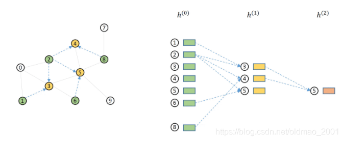
然后做对齐aligned操作:
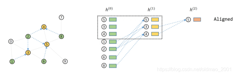
对齐之后每层节点重新排id(relabeled),然后第一层的消息传递关系保存到mfgs[0],第二层的消息传递关系保存到mfgs[1]
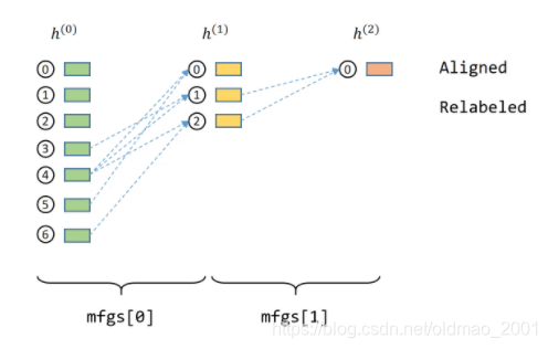
对于mfgs[0]来说,绿色方块是source nodes,黄色方块是destination nodes,可以看到为什么我们把
source nodes和destination nodes两个部分前几个节点打出来id是一样的。
建模训练
后面的模型还是用graphSAGE,然后在定义卷积层的时候要改动一下,省略了
代码我自己也没跑通,提示没装GPU版本的dgl。。。
然后重新卸载又装了一把DGL才好,估计之前装DGL没注意有专门的cuda版本
pip uninstall dgl
pip install dgl-cu102
后面代码不解释了,先贴过来:
import torch.nn as nn
import torch.nn.functional as F
from dgl.nn import SAGEConv

class Model(nn.Module):
    def __init__(self, in_feats, h_feats, num_classes):
        super(Model, self).__init__()
        self.conv1 = SAGEConv(in_feats, h_feats, aggregator_type='mean')
        self.conv2 = SAGEConv(h_feats, num_classes, aggregator_type='mean')
        self.h_feats = h_feats

    def forward(self, mfgs, x):
        # Lines that are changed are marked with an arrow: "<---"
		# 注意下面带箭头的代码和普通的卷积代码不一样
        h_dst = x[:mfgs[0].num_dst_nodes()]  # <---
        h = self.conv1(mfgs[0], (x, h_dst))  # <---
        h = F.relu(h)
        h_dst = h[:mfgs[1].num_dst_nodes()]  # <---
        h = self.conv2(mfgs[1], (h, h_dst))  # <---
        return h

model = Model(num_features, 128, num_classes).to(device)
#优化器
opt = torch.optim.Adam(model.parameters())
#加载数据
valid_dataloader = dgl.dataloading.NodeDataLoader(
    graph, valid_nids, sampler,
    batch_size=1024,
    shuffle=False,
    drop_last=False,
    num_workers=0,
    device=device
)
训练
import tqdm
import sklearn.metrics

best_accuracy = 0
best_model_path = 'model.pt'
for epoch in range(10):
    model.train()

    with tqdm.tqdm(train_dataloader) as tq:
        for step, (input_nodes, output_nodes, mfgs) in enumerate(tq):
            # feature copy from CPU to GPU takes place here
            inputs = mfgs[0].srcdata['feat']
            labels = mfgs[-1].dstdata['label']

            predictions = model(mfgs, inputs)

            loss = F.cross_entropy(predictions, labels)
            opt.zero_grad()
            loss.backward()
            opt.step()

            accuracy = sklearn.metrics.accuracy_score(labels.cpu().numpy(), predictions.argmax(1).detach().cpu().numpy())

            tq.set_postfix({'loss': '%.03f' % loss.item(), 'acc': '%.03f' % accuracy}, refresh=False)

    model.eval()

    predictions = []
    labels = []
    with tqdm.tqdm(valid_dataloader) as tq, torch.no_grad():
        for input_nodes, output_nodes, mfgs in tq:
            inputs = mfgs[0].srcdata['feat']
            labels.append(mfgs[-1].dstdata['label'].cpu().numpy())
            predictions.append(model(mfgs, inputs).argmax(1).cpu().numpy())
        predictions = np.concatenate(predictions)
        labels = np.concatenate(labels)
        accuracy = sklearn.metrics.accuracy_score(labels, predictions)
        print('Epoch {} Validation Accuracy {}'.format(epoch, accuracy))
        if best_accuracy < accuracy:
            best_accuracy = accuracy
            torch.save(model.state_dict(), best_model_path)

        # Note that this tutorial do not train the whole model to the end.
        break
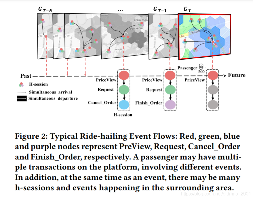
动态异质图的应用
来自滴滴团队的论文:Dynamic Heterogeneous Graph Neural Network for Real-time
Event Prediction
2020 KDD
看下面每个时序都是一个图,用GNN学到每个图的embedding,然后做成下面的序列,然后再用类似LSTM的模型处理图的embedding,然后预测出将来的embedding。


 3147
3147


 被折叠的 条评论
为什么被折叠?
被折叠的 条评论
为什么被折叠?
 到【灌水乐园】发言


