【DGL】节点分类（GCN、SAGE、自定义）

使用dgl进行节点分类（GCN）

数据集

dataset = dgl.data.CoraGraphDataset()
print("Number of categories:", dataset.num_classes)
g = dataset[0]

数据集信息：
Cora dataset，引用网络图，其中，节点表示论文，边表示论文的引用。任务是预测给定论文的类别。

NumNodes: 2708
  NumEdges: 10556
  NumFeats: 1433
  NumClasses: 7
  NumTrainingSamples: 140
  NumValidationSamples: 500
  NumTestSamples: 1000
Done loading data from cached files.
Number of categories: 7

其中，含有一个graph：

Graph(num_nodes=2708, num_edges=10556,
      ndata_schemes={'train_mask': Scheme(shape=(), dtype=torch.bool), 'label': Scheme(shape=(), dtype=torch.int64), 'val_mask': Scheme(shape=(), dtype=torch.bool), 'test_mask': Scheme(shape=(), dtype=torch.bool), 'feat': Scheme(shape=(1433,), dtype=torch.float32)}
      edata_schemes={})

train_mask: A boolean tensor indicating whether the node is in the training set.
val_mask: A boolean tensor indicating whether the node is in the validation set.
test_mask: A boolean tensor indicating whether the node is in the test set.
label: The ground truth node category.
feat: The node features.

搭建网络

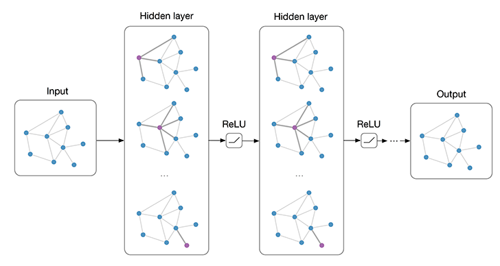
根据Graph Convolutional Network (GCN)搭建两层的图卷积神经网络。每一层通过聚合邻居节点的信息来计算新的节点表示。

class GCN(nn.Module):
    def __init__(self, in_feats, h_feats, num_classes):
        super(GCN, self).__init__()
        self.conv1 = GraphConv(in_feats, h_feats)
        self.conv2 = GraphConv(h_feats, num_classes)

    def forward(self, g, in_feat):
        h = self.conv1(g, in_feat)
        h = F.relu(h)
        h = self.conv2(g, h)
        return h

model = GCN(g.ndata['feat'].shape[1], 16, dataset.num_classes)
print(model)

数学上表示成¹：$$h_i^{(l+1)}=\sigma (b^{(l)}+\sum _{j\in \mathcal{N}(i)}\frac{1}{c_{ji}}{h}_j^{(l)}{W}^{(l)})$$

模型结构：

GCN(
  (conv1): GraphConv(in=1433, out=16, normalization=both, activation=None)
  (conv2): GraphConv(in=16, out=7, normalization=both, activation=None)
)

训练

def train(g, model):
    optimizer = torch.optim.Adam(model.parameters(), lr=0.01)
    best_val_acc = 0
    best_test_acc = 0

    features = g.ndata['feat']
    labels = g.ndata['label']
    train_mask = g.ndata['train_mask']
    val_mask = g.ndata['val_mask']
    test_mask = g.ndata['test_mask']
    for e in range(100):
        logits = model(g, features)
        pred = logits.argmax(1)
        loss = F.cross_entropy(logits[train_mask], labels[train_mask])

        train_acc = (pred[train_mask] == labels[train_mask]).float().mean()
        val_acc = (pred[val_mask] == labels[val_mask]).float().mean()
        test_acc = (pred[test_mask] == labels[test_mask]).float().mean()

        if(best_val_acc < val_acc):
            best_val_acc = val_acc
            best_test_acc = test_acc

        optimizer.zero_grad()
        loss.backward()
        optimizer.step()

        if(e%5==0):
            print(
                "In epoch {}, loss: {:.3f}, val acc: {:.3f} (best {:.3f}), test acc: {:.3f} (best {:.3f})".format(
                    e, loss, val_acc, best_val_acc, test_acc, best_test_acc
                )
            )


train(g, model)

In epoch 0, loss: 1.946, val acc: 0.240 (best 0.240), test acc: 0.254 (best 0.254)
In epoch 5, loss: 1.903, val acc: 0.642 (best 0.642), test acc: 0.639 (best 0.639)
In epoch 10, loss: 1.837, val acc: 0.696 (best 0.700), test acc: 0.711 (best 0.715)
In epoch 15, loss: 1.746, val acc: 0.674 (best 0.700), test acc: 0.685 (best 0.715)
In epoch 20, loss: 1.628, val acc: 0.694 (best 0.700), test acc: 0.710 (best 0.715)
In epoch 25, loss: 1.484, val acc: 0.690 (best 0.700), test acc: 0.715 (best 0.715)
In epoch 30, loss: 1.321, val acc: 0.710 (best 0.710), test acc: 0.732 (best 0.732)
In epoch 35, loss: 1.144, val acc: 0.714 (best 0.720), test acc: 0.738 (best 0.737)
In epoch 40, loss: 0.966, val acc: 0.730 (best 0.730), test acc: 0.742 (best 0.742)
In epoch 45, loss: 0.797, val acc: 0.742 (best 0.742), test acc: 0.745 (best 0.745)
In epoch 50, loss: 0.647, val acc: 0.756 (best 0.756), test acc: 0.756 (best 0.756)
In epoch 55, loss: 0.520, val acc: 0.762 (best 0.762), test acc: 0.759 (best 0.759)
In epoch 60, loss: 0.416, val acc: 0.768 (best 0.768), test acc: 0.767 (best 0.765)
In epoch 65, loss: 0.334, val acc: 0.762 (best 0.768), test acc: 0.771 (best 0.765)
In epoch 70, loss: 0.270, val acc: 0.758 (best 0.768), test acc: 0.774 (best 0.765)
In epoch 75, loss: 0.220, val acc: 0.760 (best 0.768), test acc: 0.777 (best 0.765)
In epoch 80, loss: 0.182, val acc: 0.764 (best 0.768), test acc: 0.779 (best 0.765)
In epoch 85, loss: 0.151, val acc: 0.764 (best 0.768), test acc: 0.780 (best 0.765)
In epoch 90, loss: 0.128, val acc: 0.764 (best 0.768), test acc: 0.782 (best 0.765)
In epoch 95, loss: 0.109, val acc: 0.766 (best 0.768), test acc: 0.779 (best 0.765)

Process finished with exit code 0

使用dgl进行节点分类（SAGE）

dgl遵循消息传递网络范式²。GraphSAGE convolution (Hamilton et al., 2017)具有以下形式：

h N ( v ) k ← A v e r a g e { h u k − 1 , ∀ u ∈ N ( v ) } h v k ← R e L U ( W k ⋅ C O N C A T ( h v k − 1 , h N ( v ) k ) ) h_\mathcal{N(v)}^k \gets Average\{ h_u ^{k-1} , \forall u \in \mathcal{N}(v) \} \\ h_v^k \gets ReLU(W^k \cdot CONCAT(h_v^{k-1}, h^k _{\mathcal{N}(v)})) hN(v)k​←Average{huk−1​,∀u∈N(v)}hvk​←ReLU(Wk⋅CONCAT(hvk−1​,hN(v)k​))

实现SAGE

在dgl中有内置的SAGEConv。下面来自己实现：

class SAGEConv(nn.Module):
    def __init__(self, in_feat, out_feat):
        super(SAGEConv, self).__init__()
        # A linear submodule for projecting the input and neighbor feature to the output.
        self.linear = nn.Linear(in_feat*2, out_feat) # W

    def forward(self, g, h):
        with g.local_scope():#在这个区域内对g的修改不会同步到原始的图上
            g.ndata['h'] = h
            g.update_all(    #对所有的节点和边采用下面的message函数和reduce函数
                message_func=fn.copy_u("h", "m"), #message函数：将节点特征'h'作为消息传递给邻居，命名为'm'
                reduce_func=fn.mean("m", "h_N"),  #reduce函数：将接收到的'm'信息取平均，保存至节点特征'h_N'
            )
            h_N = g.ndata["h_N"]
            h_total = torch.cat([h, h_N], dim=1)
            return self.linear(h_total)

依此搭建新的网络：

class Model(nn.Module):
    def __init__(self, in_feats, h_feats, num_classes):
        super(Model, self).__init__()
        self.conv1 = SAGEConv(in_feats, h_feats)
        self.conv2 = SAGEConv(h_feats, num_classes)
    def forward(self, g, in_feat):
        h = self.conv1(g, in_feat)
        h = F.relu(h)
        h = self.conv2(g, h)
        return h

model = Model(g.ndata['feat'].shape[1], 16, dataset.num_classes)

效果和GCN差不多吧

引入边权

class WeightedSAGEConv(nn.Module):
    def __init__(self, in_feat, out_feat):
        super(WeightedSAGEConv, self).__init__()
        # A linear submodule for projecting the input and neighbor feature to the output.
        self.linear = nn.Linear(in_feat * 2, out_feat)

    def forward(self, g, h, w):
        with g.local_scope():
            g.ndata["h"] = h
            g.edata["w"] = w
            g.update_all(
                message_func=fn.u_mul_e("h", "w", "m"), #节点特征'h' 与 邻居间的边特征'w' 的乘积作为消息传递给邻居，记作'm'
                reduce_func=fn.mean("m", "h_N"), #将接收到的'm'信息取平均，保存至节点特征'h_N'
            )
            h_N = g.ndata["h_N"]
            h_total = torch.cat([h, h_N], dim=1)
            return self.linear(h_total)


class Model(nn.Module):
    def __init__(self, in_feats, h_feats, num_classes):
        super(Model, self).__init__()
        self.conv1 = WeightedSAGEConv(in_feats, h_feats)
        self.conv2 = WeightedSAGEConv(h_feats, num_classes)

    def forward(self, g, in_feat):
        h = self.conv1(g, in_feat, torch.ones(g.num_edges(), 1).to(g.device))#数据中没有边特征，在这里手动添加
        h = F.relu(h)
        h = self.conv2(g, h, torch.ones(g.num_edges(), 1).to(g.device))
        return h


model = Model(g.ndata["feat"].shape[1], 16, dataset.num_classes)

更多自定义操作

见dgl.function

内置函数 dgl.function.u_add_v('hu'，'hv'，' he')等价于：

def message_func(edges):#返回值为字典形式
    return {'he': edges.src['hu'] + edges.dst['hv']}

---

1. https://docs.dgl.ai/generated/dgl.nn.pytorch.conv.GraphConv.html#dgl.nn.pytorch.conv.GraphConv ↩︎

2. Neural Message Passing for Quantum Chemistry ↩︎