


Lenet-5是Yann LeCun提出的,对MNIST数据集的分识别准确度可达99.2%。下面简要介绍下每层的结构:
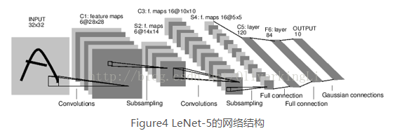
第一层:卷积层
该层的输入是原始图像的像素值,以MNIST数据集为例,则是28x28x1,第一层过滤器尺寸为5x5,深度设置为6,不适用0去填充,因此该层的输出尺寸是28-5+1=24,深度也为6.
第二层:池化层
接受第一层的输出作为输入,过滤器大小选为2x2,步长2.
第三层:卷积层
卷积和大小5x5,深度为16,同样不使用0填充,步长为1.
第四层:池化层
卷积核采用2x2,步长2
第五层:全连接
卷积核为5x5,输出节点为120
第六层:全连接层
输入节点数120,输出节点数84
第七层:全连接层
输入84,输出10
Hinton的学生Alex Krizhevsky提出来深度卷积模型Alexnet,这是一种更深的更宽的版本。该模型在ILSVRS 2012年的比赛中一举夺冠,top-5错误的概率下降到16.4%,识别的准确度有了质的飞跃,从而刮起了深度卷积学习之热。
一:概念原理介绍
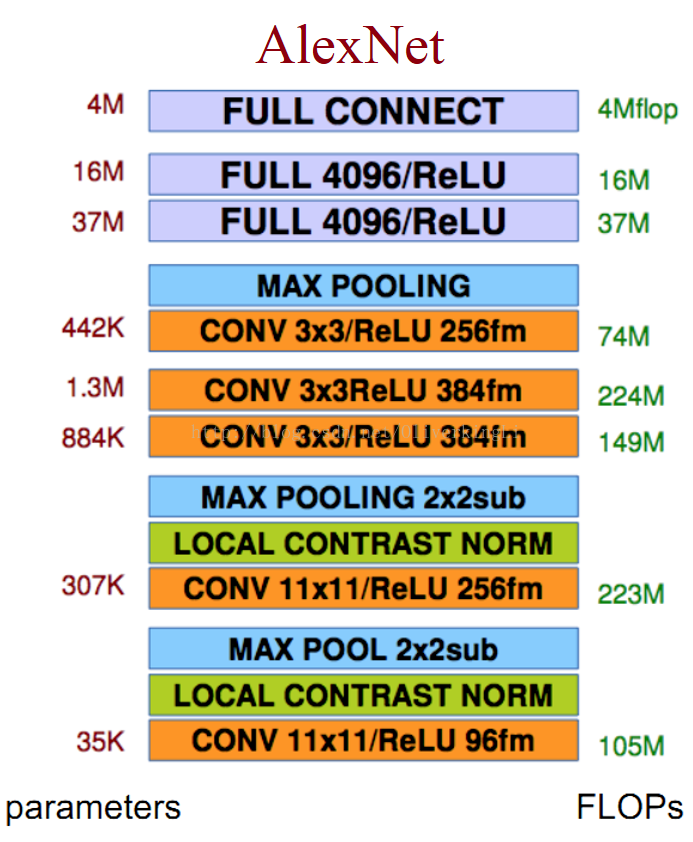
Alexnet包含了6亿3000万个连接,6000万个参数和65万个神经元,拥有5个卷积层,其中三个卷积层后面连接了最大池化层,最后还包括3个全连接层。
下面介绍一下Alexnet的思想:
1.成功使用ReLU作为CNN的激活函数,而且验证了深度学习模型在更深的网络上其效果较之于Sigmoid有了极大的提高,成功解决了Sigmoid在网络较深的时候出现的梯度弥散的问题(也就是常说的梯度消失)。
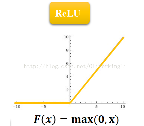
当进来的输入小于0时将其全部置0,这样模拟生物学上神经元的信号抑制,只有信号的刺激达到一定的阈值后才足够引起兴奋。
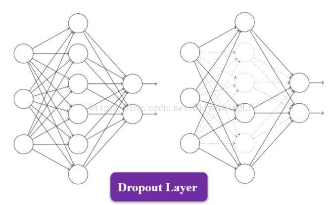
2.训练数据集的时候加入Dropout随机忽略一部分的神经元,从而避免模型的过拟合问题。由于加入dropoutzai模型学习过程中,随机丢弃部分过于细致的特征是很有必要的,这样模型学习到的是明显的特征,从而增加模型的泛化能力。在Alexnet中主要是后面的几个全连接层使用。
3.在CNN模型中,使用重叠的最大赤化。在这以前大部分是使用平均池化,到了Alexnet中就全部使用最大池化(max pool),这可以很好的解决平均池化的模糊问题。同时Alexnet提出让卷积核扫描步长比池化核的尺寸小,这样在池化层的输出之间会有重叠和覆盖,在一定程度上提升了特征的丰富性。
4.提出了LRN层概念并加入应用。LRN又叫局部响应归一化,具有对局部神经元的活动创建竞争机制,使得其中响应比较大的值变得更大,而对响应比较小的值更加加以抑制,从而增强模型的泛化能力,这和让更加明显的特征更加明显,很细微不明显的特征加以抑制是一个道理。
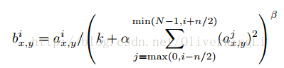
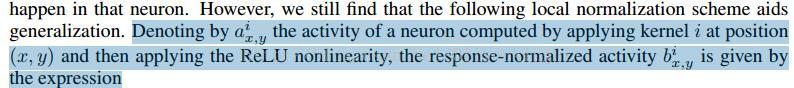
大意是:i表示第i个核在位置(x,y)运用激活函数ReLU后的输出,n是同一位置上临近的kernal map的数目,N是kernal的总数。参数K,n,alpha,belta都是超参数,一般设置k=2,n=5,aloha=1*e-4,beta=0.75
网络模型如下所示:
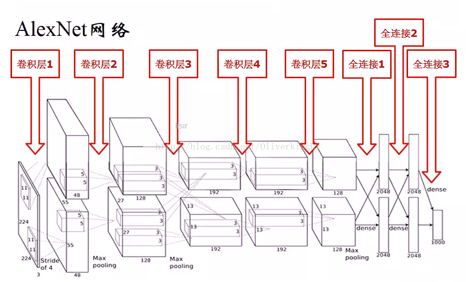
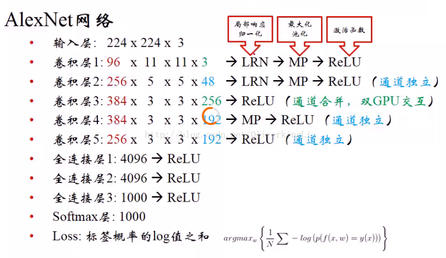
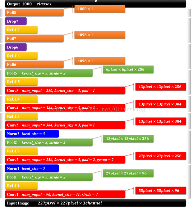
整个Alexnet具有8个需要训练参数的层(不包括有max pool以及LRN层),前面5个是卷积层,后面的3个是全链接层。如上图。最后的一层是1000类的输出的softmax层,是作为最后分类输出的。LRN出现在第一和第二个卷积层之后,max pool出现在两个LRN层以及最后一个卷积层之后。而ReLU均出现在这8层每一层的后面。Alexnet在训练时候分到两个GPU加以训练,两个GPU除了在第3层卷积层进行数据通信外,其他的卷积操作(提取特征)都是独立进行。那么下面就介绍一个通道上的GPU就可:
一开始ALexnet比赛时候使用的是224x224x3的图片输入,第一个卷积层使用卷积核是96(个数)x11x11x3,步长是4;接着LRN层;然后是3x3的max pool,步长是2。之后的卷积层卷积核尺寸都比较小,5x5或者3x3,步长为2。下面给出几个公式用于计算每一层的参数:
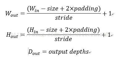
例如对于第一个卷积层conv1:
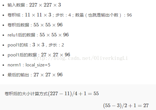
故此根据公式计算得到的各个层的具体参数如下:
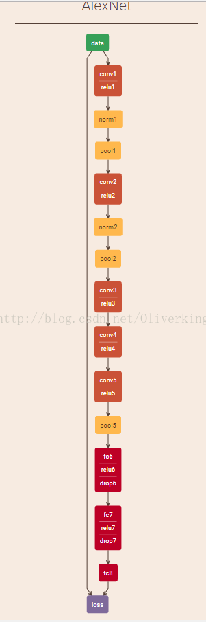
整个的Alexnet网络结构可以描述为:
当然如果你需要更加详细的网络结构图:
可以查看:http://ethereon.github.io/netscope/#/gist/e65799e70358c6782b1b
二:基于tensorflow代码实现以及调参对比
首先实现一个lenet-5的代码
import tensorflow as tf
import input_data

mnist = input_data.read_data_sets('MNIST_data', one_hot=True)

sess = tf.InteractiveSession()

# 训练数据
x = tf.placeholder("float", shape=[None, 784])
# 训练标签数据
y_ = tf.placeholder("float", shape=[None, 10])
# 把x更改为4维张量,第1维代表样本数量,第2维和第3维代表图像长宽, 第4维代表图像通道数, 1表示黑白
x_image = tf.reshape(x, [-1, 28, 28, 1])

# 第一层:卷积层
# 过滤器大小为5*5, 当前层深度为1, 过滤器的深度为32
conv1_weights = tf.get_variable("conv1_weights", [5, 5, 1, 32], initializer=tf.truncated_normal_initializer(stddev=0.1))
conv1_biases = tf.get_variable("conv1_biases", [32], initializer=tf.constant_initializer(0.0))
# 移动步长为1, 使用全0填充
conv1 = tf.nn.conv2d(x_image, conv1_weights, strides=[1, 1, 1, 1], padding='SAME')
# 激活函数Relu去线性化
relu1 = tf.nn.relu(tf.nn.bias_add(conv1, conv1_biases))

#第二层:最大池化层
#池化层过滤器的大小为2*2, 移动步长为2,使用全0填充
pool1 = tf.nn.max_pool(relu1, ksize=[1, 2, 2, 1], strides=[1, 2, 2, 1], padding='SAME')

#第三层:卷积层
conv2_weights = tf.get_variable("conv2_weights", [5, 5, 32, 64], initializer=tf.truncated_normal_initializer(stddev=0.1)) #过滤器大小为5*5, 当前层深度为32, 过滤器的深度为64
conv2_biases = tf.get_variable("conv2_biases", [64], initializer=tf.constant_initializer(0.0))
conv2 = tf.nn.conv2d(pool1, conv2_weights, strides=[1, 1, 1, 1], padding='SAME') #移动步长为1, 使用全0填充
relu2 = tf.nn.relu( tf.nn.bias_add(conv2, conv2_biases) )

#第四层:最大池化层
#池化层过滤器的大小为2*2, 移动步长为2,使用全0填充
pool2 = tf.nn.max_pool(relu2, ksize=[1, 2, 2, 1], strides=[1, 2, 2, 1], padding='SAME')

#第五层:全连接层
fc1_weights = tf.get_variable("fc1_weights", [7 * 7 * 64, 1024], initializer=tf.truncated_normal_initializer(stddev=0.1)) #7*7*64=3136把前一层的输出变成特征向量
fc1_baises = tf.get_variable("fc1_baises", [1024], initializer=tf.constant_initializer(0.1))
pool2_vector = tf.reshape(pool2, [-1, 7 * 7 * 64])
fc1 = tf.nn.relu(tf.matmul(pool2_vector, fc1_weights) + fc1_baises)

#为了减少过拟合,加入Dropout层
keep_prob = tf.placeholder(tf.float32)
fc1_dropout = tf.nn.dropout(fc1, keep_prob)

#第六层:全连接层
fc2_weights = tf.get_variable("fc2_weights", [1024, 10], initializer=tf.truncated_normal_initializer(stddev=0.1)) #神经元节点数1024, 分类节点10
fc2_biases = tf.get_variable("fc2_biases", [10], initializer=tf.constant_initializer(0.1))
fc2 = tf.matmul(fc1_dropout, fc2_weights) + fc2_biases

#第七层:输出层
# softmax
y_conv = tf.nn.softmax(fc2)

#定义交叉熵损失函数
cross_entropy = tf.reduce_mean(-tf.reduce_sum(y_ * tf.log(y_conv), reduction_indices=[1]))

#选择优化器,并让优化器最小化损失函数/收敛, 反向传播
train_step = tf.train.AdamOptimizer(1e-4).minimize(cross_entropy)

# tf.argmax()返回的是某一维度上其数据最大所在的索引值,在这里即代表预测值和真实值
# 判断预测值y和真实值y_中最大数的索引是否一致,y的值为1-10概率
correct_prediction = tf.equal(tf.argmax(y_conv,1), tf.argmax(y_,1))

# 用平均值来统计测试准确率
accuracy = tf.reduce_mean(tf.cast(correct_prediction, tf.float32))

#开始训练
sess.run(tf.global_variables_initializer())
for i in range(10000):
    batch = mnist.train.next_batch(100)
    if i%100 == 0:
        train_accuracy = accuracy.eval(feed_dict={x:batch[0], y_: batch[1], keep_prob: 1.0}) #评估阶段不使用Dropout
        print("step %d, training accuracy %g" % (i, train_accuracy))
    train_step.run(feed_dict={x: batch[0], y_: batch[1], keep_prob: 0.5}) #训练阶段使用50%的Dropout


#在测试数据上测试准确率
print("test accuracy %g" % accuracy.eval(feed_dict={x: mnist.test.images, y_: mnist.test.labels, keep_prob: 1.0}))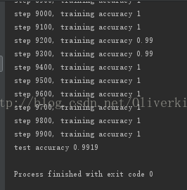
一个缩小版的alexnet,主要采用alexnet设计,但不是标准的alexnet结
# -*- coding: utf-8 -*-
from __future__ import print_function
from __future__ import absolute_import
from __future__ import division

import argparse
import sys

import input_data
import tensorflow as tf

mnist = input_data.read_data_sets("MNIST_data", one_hot=True)

# 定义网络超参数
learning_rate = 1e-4
training_iters = 300000
batch_size = 64
display_step = 20

# 定义网络参数
n_input = 784 # 输入的维度
n_classes = 10 # 标签的维度
dropout = 0.5 # Dropout 的概率

# 占位符输入
x = tf.placeholder(tf.float32, [None, n_input])
y = tf.placeholder(tf.float32, [None, n_classes])
keep_prob = tf.placeholder(tf.float32)

# 卷积操作
def conv2d(name, l_input, w, b, k):
    return tf.nn.relu(tf.nn.bias_add(tf.nn.conv2d(l_input,
                                                  w, strides=[1, k, k, 1],
                                                  padding='SAME'), b), name=name)

# 最大下采样操作
def max_pool(name, l_input, k1, k2):
    return tf.nn.max_pool(l_input, ksize=[1, k1, k1, 1], strides=[1, k2, k2, 1], padding='SAME', name=name)

# 归一化操作
def norm(name, l_input, lsize=4):
    return tf.nn.lrn(l_input, lsize, bias=1.0, alpha=0.001 / 9.0, beta=0.75, name=name)

# 定义整个网络
def alex_net(_X, _weights, _biases, _dropout):
    # 向量转为矩阵
    _X = tf.reshape(_X, shape=[-1, 28, 28, 1])

    # 卷积层
    conv1 = conv2d('conv1', _X, _weights['wc1'], _biases['bc1'], 2)

    # 归一化层
    norm1 = norm('norm1', conv1, lsize=4)
    # 下采样层
    pool1 = max_pool('pool1', norm1, k1=3, k2=2)
    # Dropout
    norm1 = tf.nn.dropout(pool1, _dropout)

    # 卷积
    conv2 = conv2d('conv2', norm1, _weights['wc2'], _biases['bc2'], 1)
    # 归一化
    norm2 = norm('norm2', conv2, lsize=4)
    # 下采样
    pool2 = max_pool('pool2', norm2, k1=3, k2=2)
    # Dropout
    norm2 = tf.nn.dropout(pool2, _dropout)

    # 卷积
    conv3 = conv2d('conv3', norm2, _weights['wc3'], _biases['bc3'], 1)
    # 归一化384
    norm3 = norm('norm3', conv3, lsize=4)
    # 下采样
    # pool3 = max_pool('pool3', norm3, k=2)
    # Dropoutize of tensor shape you provided is 150528 : 224x224x
    norm3 = tf.nn.dropout(norm3, _dropout)
    '''
    # 卷积
    conv4 = conv2d('conv4', norm3, _weights['wc4'], _biases['bc4'], 1)
    # 归一化
    norm4 = norm('norm4', conv4, lsize=4)
    # 下采样
    # pool3 = max_pool('pool3', norm3, k=2)
    # Dropout
    norm4 = tf.nn.dropout(norm4, _dropout)

    # 卷积
    conv5 = conv2d('conv5', norm4, _weights['wc5'], _biases['bc5'], 1)
    # 归一化256
    norm5 = norm('norm5', conv5, lsize=4)
    # 下采样
    pool5 = max_pool('pool5', norm5, k1=3, k2=2)
    # Dropout
    norm5 = tf.nn.dropout(pool5, _dropout)
    '''
    # 全连接层,先把特征图转为向量
    dense1 = tf.reshape(norm3, [-1, _weights['wd1'].get_shape().as_list()[0]])
    dense1 = tf.nn.dropout(tf.nn.relu(tf.matmul(dense1, _weights['wd1']) + _biases['bd1'], name='fc1'), _dropout)
    # 全连接层4096
    dense2 = tf.nn.relu(tf.matmul(dense1, _weights['wd2']) + _biases['bd2'], name='fc2') # Relu activation

    # 网络输出层384
    out = tf.matmul(dense2, _weights['out']) + _biases['out']
    return out

# 存储所有的网络参数48
'''
weights = {
    'wc1': tf.Variable(tf.random_normal([3, 3, 1, 64])),
    'wc2': tf.Variable(tf.random_normal([3, 3, 64, 128])),
    'wc3': tf.Variable(tf.random_normal([3, 3, 128, 256])),
    'wd1': tf.Variable(tf.random_normal([4*4*256, 1024])),
    'wd2': tf.Variable(tf.random_normal([1024, 1024])),
    'out': tf.Variable(tf.random_normal([1024, 10]))
}
biases = {
    'bc1': tf.Variable(tf.random_normal([64])),
    'bc2': tf.Variable(tf.random_normal([128])),
    'bc3': tf.Variable(tf.random_normal([256])),
    'bd1': tf.Variable(tf.random_normal([1024])),
    'bd2': tf.Variable(tf.random_normal([1024])),
    'out': tf.Variable(tf.random_normal([n_classes]))
}
'''
# 以字典的形式设置权重和偏置
weights = {
    'wc1': tf.Variable(tf.random_normal([3, 3, 1, 64])),
    'wc2': tf.Variable(tf.random_normal([3, 3, 64, 128])),
    'wc3': tf.Variable(tf.random_normal([3, 3, 128, 256])),
    'wd1': tf.Variable(tf.random_normal([4*4*256, 1024])),
    'wd2': tf.Variable(tf.random_normal([1024, 1024])),
    'out': tf.Variable(tf.random_normal([1024, 10]))
}
biases = {
    'bc1': tf.Variable(tf.random_normal([64])),
    'bc2': tf.Variable(tf.random_normal([128])),
    'bc3': tf.Variable(tf.random_normal([256])),
    'bd1': tf.Variable(tf.random_normal([1024])),
    'bd2': tf.Variable(tf.random_normal([1024])),
    'out': tf.Variable(tf.random_normal([n_classes]))
}

# 构建模型
pred = alex_net(x, weights, biases, keep_prob)

# 定义损失函数和学习步骤
cost = tf.reduce_mean(tf.nn.softmax_cross_entropy_with_logits(logits=pred, labels=y))
optimizer = tf.train.AdamOptimizer(1e-4).minimize(cost)

# 测试网络
correct_pred = tf.equal(tf.argmax(pred, 1), tf.argmax(y, 1))
accuracy = tf.reduce_mean(tf.cast(correct_pred, tf.float32))

# 初始化所有的共享变量
init = tf.initialize_all_variables()

# 开启一个训练
with tf.Session() as sess:
    sess.run(init)
    step = 1
    # Keep training until reach max iterations
    while step * batch_size < training_iters:
        batch_xs, batch_ys = mnist.train.next_batch(batch_size)
        # 获取批数据
        sess.run(optimizer, feed_dict={x: batch_xs, y: batch_ys, keep_prob: dropout})
        if step % display_step == 0:
            # 计算精度
            acc = sess.run(accuracy, feed_dict={x: batch_xs, y: batch_ys, keep_prob: 1.})
            # 计算损失值
            loss = sess.run(cost, feed_dict={x: batch_xs, y: batch_ys, keep_prob: 1.})
            print("Iter " + str(step*batch_size) + ", Minibatch Loss= " + "{:.6f}".format(loss) +
                   ", Training Accuracy = " + "{:.5f}".format(acc))
        step += 1
    print("Optimization Finished!")
    # 计算测试精度
    print("Testing Accuracy:", sess.run(accuracy, feed_dict={x: mnist.test.images[:256],
                                                             y: mnist.test.labels[:256],
                                                             keep_prob: 0.5}))
    print('**********************')
    print("Testing Accuracy:", sess.run(accuracy, feed_dict={x: mnist.test.images[:256],
                                                             y: mnist.test.labels[:256],
                                                             keep_prob: 1.0}))

# Merge all the summaries and write them out to
  # /tmp/tensorflow/mnist/logs/mnist_with_summaries (by default)


 1651
1651

 被折叠的 条评论
为什么被折叠?
被折叠的 条评论
为什么被折叠?
 到【灌水乐园】发言


