


本系列为MIT Gilbert Strang教授的"数据分析、信号处理和机器学习中的矩阵方法"的学习笔记。
- Gilbert Strang & Sarah Hansen | Sprint 2018
- 18.065: Matrix Methods in Data Analysis, Signal Processing, and Machine Learning
- 视频网址: https://ocw.mit.edu/courses/18-065-matrix-methods-in-data-analysis-signal-processing-and-machine-learning-spring-2018/
- 关注下面的公众号,回复“ 矩阵方法 ”,即可获取 本系列完整的pdf笔记文件~
内容在CSDN、知乎和微信公众号同步更新

- Markdown源文件暂未开源,如有需要可联系邮箱
- 笔记难免存在问题,欢迎联系邮箱指正
Lecture 0: Course Introduction
Lecture 1 The Column Space of A A A Contains All Vectors A x Ax Ax
Lecture 2 Multiplying and Factoring Matrices
Lecture 3 Orthonormal Columns in Q Q Q Give Q ′ Q = I Q'Q=I Q′Q=I
Lecture 4 Eigenvalues and Eigenvectors
Lecture 5 Positive Definite and Semidefinite Matrices
Lecture 6 Singular Value Decomposition (SVD)
Lecture 7 Eckart-Young: The Closest Rank k k k Matrix to A A A
Lecture 8 Norms of Vectors and Matrices
Lecture 9 Four Ways to Solve Least Squares Problems
Lecture 10 Survey of Difficulties with A x = b Ax=b Ax=b
Lecture 11 Minimizing ||x|| Subject to A x = b Ax=b Ax=b
Lecture 12 Computing Eigenvalues and Singular Values
Lecture 13 Randomized Matrix Multiplication
Lecture 14 Low Rank Changes in A A A and Its Inverse
Lecture 15 Matrices A ( t ) A(t) A(t) Depending on t t t, Derivative = d A / d t dA/dt dA/dt
Lecture 16 Derivatives of Inverse and Singular Values
Lecture 17 Rapidly Decreasing Singular Values
Lecture 18 Counting Parameters in SVD, LU, QR, Saddle Points
Lecture 19 Saddle Points Continued, Maxmin Principle
Lecture 20 Definitions and Inequalities
Lecture 21 Minimizing a Function Step by Step
Lecture 22 Gradient Descent: Downhill to a Minimum
Lecture 23 Accelerating Gradient Descent (Use Momentum)
Lecture 24 Linear Programming and Two-Person Games
Lecture 25 Stochastic Gradient Descent
Lecture 26 Structure of Neural Nets for Deep Learning
Lecture 27 Backpropagation: Find Partial Derivatives
Lecture 28 Computing in Class [No video available]
Lecture 29 Computing in Class (cont.) [No video available]
Lecture 30 Completing a Rank-One Matrix, Circulants!
Lecture 31 Eigenvectors of Circulant Matrices: Fourier Matrix
Lecture 32 ImageNet is a Convolutional Neural Network (CNN), The Convolution Rule
Lecture 33 Neural Nets and the Learning Function
Lecture 34 Distance Matrices, Procrustes Problem
Lecture 35 Finding Clusters in Graphs
Lecture 36 Alan Edelman and Julia Language
文章目录
Lecture 3: Orthonormal Columns in Q Q Q Give Q ′ Q = I Q'Q = I Q′Q=I
Today:
- Matrices Q Q Q: have orthonormal columns
The Definition of Orthogonal Matrix
- Q has Orthonormal Columns
- A = [ q 1 , q 2 , . . . , q n ] A = \begin{bmatrix} q_1, q_2, ..., q_n \end{bmatrix} A=[q1,q2,...,qn]
- 其中 q i q_i qi 为 Orthonormal Columns
-
Q
T
Q
=
I
Q^T Q = I
QTQ=I
- Proof: Q T Q = [ q 1 T q 2 T ⋅ ⋅ ⋅ q n T ] [ q 1 , q 2 , . . . , q n ] = [ 1 , 0 , . . . , 0 0 , 1 , . . . , 0 . . . 0 , 0 , . . . , 1 ] = I Q^T Q = \begin{bmatrix} q_1^T \\ q_2^T \\ \cdot \cdot \cdot \\ q_n^T \end{bmatrix}\begin{bmatrix} q_1, q_2, ..., q_n \end{bmatrix} = \begin{bmatrix} 1, 0, ..., 0 \\ 0, 1, ..., 0 \\ ... \\ 0, 0, ..., 1 \end{bmatrix} = I QTQ=⎣⎢⎢⎡q1Tq2T⋅⋅⋅qnT⎦⎥⎥⎤[q1,q2,...,qn]=⎣⎢⎢⎡1,0,...,00,1,...,0...0,0,...,1⎦⎥⎥⎤=I
- I I I中的0:Ortho part
- I I I中的diagonal 1: normal part
- Question 1:
Q
Q
T
=
I
Q Q^T = I
QQT=I ??
- 不一定,sometimes yes sometimes no
- Yes:
Q
Q
T
=
I
Q Q^T = I
QQT=I
- when Q is square
- 因为, Q Q Q是方阵 + Q T Q = I Q^T Q = I QTQ=I ⇒ \Rightarrow ⇒ Q Q Q可逆且$Q^{-1} = Q^T $ ⇒ \Rightarrow ⇒ Q Q T = I Q Q^T = I QQT=I
- 此时Q常被称为 “Orthogonal Matrix”
- 正交矩阵 (若推广到复数域,则为酉矩阵)
Examples of Orthogonal Matrix
- Square Q: 正交矩阵!Orthogonal Matrix
- Square
Q
=
[
c
o
s
θ
,
−
s
i
n
θ
s
i
n
θ
,
c
o
s
θ
]
Q = \begin{bmatrix} cos \theta, -sin \theta \\ sin \theta, cos \theta \end{bmatrix}
Q=[cosθ,−sinθsinθ,cosθ]
- This is a Rotation Matrix
- a rotation of the whole plane by theta
- [ c o s θ , − s i n θ s i n θ , c o s θ ] [ 1 0 ] = [ c o s θ s i n θ ] \begin{bmatrix} cos \theta, -sin \theta \\ sin \theta, cos \theta \end{bmatrix}\begin{bmatrix} 1 \\ 0 \end{bmatrix} = \begin{bmatrix} cos \theta \\ sin \theta \end{bmatrix} [cosθ,−sinθsinθ,cosθ][10]=[cosθsinθ]
- This is a Rotation Matrix
- 正交矩阵
Q
Q
Q Property 1:长度不变
- It does not change length
- ∥ x ∥ = ∥ Q x ∥ , ∀ x \|x\| = \| Qx\|, \forall x ∥x∥=∥Qx∥,∀x
- 这也是一个原因that orthogonal matrix is so much loved
- Proof:
- 重点: x T x x^T x xTx = ∥ x ∥ 2 2 \|x\|_2^2 ∥x∥22
- 因此:
- ∥ Q x ∥ 2 2 = ( Q x ) T ( Q x ) = x T Q T Q x = x T x = ∥ x ∥ 2 2 \| Qx\|_2^2 = (Qx)^T(Qx)=x^TQ^TQx = x^Tx = \|x\|_2^2 ∥Qx∥22=(Qx)T(Qx)=xTQTQx=xTx=∥x∥22
- 证毕
- Please note again:
- When we say “orthogonal matrix”, we mean that it is orthonormal!
- Q T Q = Q Q T = I Q^T Q = Q Q^T = I QTQ=QQT=I ( Q T = Q − 1 Q^T = Q^{-1} QT=Q−1)
- Square
Q
=
[
c
o
s
θ
,
−
s
i
n
θ
s
i
n
θ
,
c
o
s
θ
]
Q = \begin{bmatrix} cos \theta, -sin \theta \\ sin \theta, cos \theta \end{bmatrix}
Q=[cosθ,−sinθsinθ,cosθ]

More examples of Otrhogonal Matrix Q Q Q
- 1 (见上):Rotation Matrix
- 2: Reflection Matrix
- 3: Householder Reflections Matrix
- We are collecting together some orthogonal matrices that are useful and important.
- Householder found a whole bunch of them – 很重要
- 4: Hadmard Matrix
- Example 1:
Q
=
[
c
o
s
θ
s
i
n
θ
s
i
n
θ
−
c
o
s
θ
]
Q = \begin{bmatrix} cos \theta & sin \theta \\ sin \theta & -cos \theta \end{bmatrix}
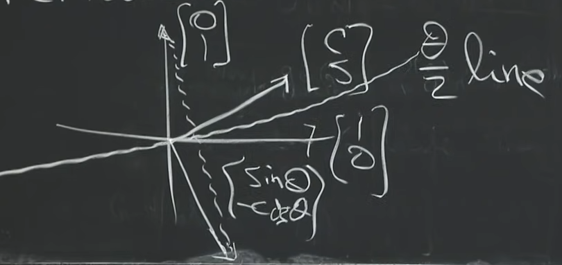
Q=[cosθsinθsinθ−cosθ]
- not a rotation anymore
- This a Reflection Matrix 见下图
-
Q
x
=
[
c
o
s
θ
s
i
n
θ
s
i
n
θ
−
c
o
s
θ
]
[
1
0
]
=
[
c
o
s
θ
s
i
n
θ
]
Qx = \begin{bmatrix} cos \theta & sin \theta \\ sin \theta & -cos \theta \end{bmatrix}\begin{bmatrix} 1 \\ 0 \end{bmatrix} = \begin{bmatrix} cos \theta \\ sin \theta \end{bmatrix}
Qx=[cosθsinθsinθ−cosθ][10]=[cosθsinθ]
- 关于line ∠ = θ / 2 \angle = \theta/2 ∠=θ/2 对称
-
Q
x
=
[
c
o
s
θ
s
i
n
θ
s
i
n
θ
−
c
o
s
θ
]
[
0
1
]
=
[
s
i
n
θ
−
c
o
s
θ
]
Qx = \begin{bmatrix} cos \theta & sin \theta \\ sin \theta & -cos \theta \end{bmatrix}\begin{bmatrix} 0 \\ 1 \end{bmatrix} = \begin{bmatrix} sin \theta \\ -cos \theta \end{bmatrix}
Qx=[cosθsinθsinθ−cosθ][01]=[sinθ−cosθ]
- 关于line ∠ = θ / 2 \angle = \theta/2 ∠=θ/2 对称
-
Q
x
=
[
c
o
s
θ
s
i
n
θ
s
i
n
θ
−
c
o
s
θ
]
[
1
0
]
=
[
c
o
s
θ
s
i
n
θ
]
Qx = \begin{bmatrix} cos \theta & sin \theta \\ sin \theta & -cos \theta \end{bmatrix}\begin{bmatrix} 1 \\ 0 \end{bmatrix} = \begin{bmatrix} cos \theta \\ sin \theta \end{bmatrix}
Qx=[cosθsinθsinθ−cosθ][10]=[cosθsinθ]
-
Example 2: Householder reflections
- Start with u T u = 1 u^T u = 1 uTu=1
- Then, created this matrix:
-
H
=
I
−
2
u
u
T
H = I - 2 u u^T
H=I−2uuT
- u u T u u^T uuT: a column times a row
-
H
=
I
−
2
u
u
T
H = I - 2 u u^T
H=I−2uuT
- H’s properties:
- 1 Symmetric
- both I I I and u u T u u ^T uuT are symmetric
- H = H T H = H^T H=HT ⇒ \Rightarrow ⇒ H T H = H H T H^T H = H H ^T HTH=HHT
- 2 Orthogonal
-
H
T
H
=
H
H
=
(
I
−
2
u
u
T
)
(
I
−
2
u
u
T
)
=
I
−
4
u
u
T
+
4
u
u
T
u
u
T
=
I
H^T H = H H = (I - 2 u u^T) (I - 2 u u^T) = I - 4 u u^T + 4 u u ^T u u ^T = I
HTH=HH=(I−2uuT)(I−2uuT)=I−4uuT+4uuTuuT=I
- just a dinky dinky 小的,小而整洁的,无关紧要的
-
H
T
H
=
H
H
=
(
I
−
2
u
u
T
)
(
I
−
2
u
u
T
)
=
I
−
4
u
u
T
+
4
u
u
T
u
u
T
=
I
H^T H = H H = (I - 2 u u^T) (I - 2 u u^T) = I - 4 u u^T + 4 u u ^T u u ^T = I
HTH=HH=(I−2uuT)(I−2uuT)=I−4uuT+4uuTuuT=I
- 1 Symmetric
-
Example 3: Hadamard Matrix+
- 2阶Hadamard Matrix: H 2 = [ 1 1 1 − 1 ] H_2 = \begin{bmatrix} 1 & 1 \\ 1 & -1 \end{bmatrix} H2=[111−1]
- 4阶Hadamard Matrix: H 4 = [ 1 1 1 1 1 − 1 1 − 1 1 1 − 1 − 1 1 − 1 − 1 1 ] = [ H 2 H 2 H 2 − H 2 ] H_4 = \begin{bmatrix} 1 & 1 & 1 & 1 \\ 1 & -1 & 1 & -1 \\ 1 & 1 & -1 & -1 \\ 1 & -1 & -1 & 1 \\ \end{bmatrix} = \begin{bmatrix} H_2 & H_2 \\ H_2 & -H_2 \\ \end{bmatrix} H4=⎣⎢⎢⎡11111−11−111−1−11−1−11⎦⎥⎥⎤=[H2H2H2−H2]
- 8阶 Hadamard Matrix:
- H 8 = [ H 4 H 4 H 4 − H 4 ] H_8 = \begin{bmatrix} H_4 & H_4 \\ H_4 & -H_4 \\ \end{bmatrix} H8=[H4H4H4−H4]
- 12阶 Hadamard Matrix:
- 存在
- 要求:
- Hadamard矩阵的阶数N 必须是4的倍数
- 若要使其成为Orthogonal Matrix, 需乘以归一化常数,使其满足 H T H = I H^T H = I HTH=I;否则 H T H = n I H^T H = nI HTH=nI
Where does Orthogonal Matrix comes from?
- Orthogonal vectors 会在什么地方in math 出现?
-
1 They could be the eigenvectors of symmetric matrix
- 正交矩阵的一个重要来源
- 构造一个正交矩阵非常容易:随便找一个对称矩阵,its eigenvectors are automatically orthogonal
- 下一节课将会大量涉及,这里是基础
- Matrix Q (eigenvectors of symmetric matrix S = S T S = S^T S=ST) are orthogonal
- 此外: Eigenvectors of Q 也是离散傅里叶变换的基础
- Eigenvectors of Q = [ 0 1 0 0 0 0 1 0 0 0 0 1 1 0 0 0 ] Q = \begin{bmatrix} 0 & 1 & 0 & 0 \\ 0 & 0 & 1 & 0 \\ 0 & 0 & 0 & 1 \\ 1 & 0 & 0 & 0 \end{bmatrix} Q=⎣⎢⎢⎡0001100001000010⎦⎥⎥⎤ are Fourier Discrete Transform
- 下面计算 Q Q Q的特征向量:
- F 4 = F_4 = F4= eigenvectors of Q Q Q = [ 1 1 1 1 1 i i 2 i 3 1 i 2 i 4 i 6 1 i 3 i 6 i 9 ] \begin{bmatrix} 1 & 1 & 1 & 1 \\ 1 & i & i^2 & i^3 \\ 1 & i^2 & i^4 & i^6 \\ 1 & i^3 & i^6 & i^9 \end{bmatrix} ⎣⎢⎢⎡11111ii2i31i2i4i61i3i6i9⎦⎥⎥⎤
-
F
4
F_4
F4也是正交的!
- 逐列相乘即可证明 (需共轭)
- c o l i ^ ⋅ c o l j \hat{col_{i}} \cdot col_{j} coli^⋅colj
- 正交矩阵不同特征值对应的特征向量彼此(共轭)正交 (证明简单,略)
- 思路:
- 第一列:Q为permute matrix, Q x = λ x Qx = \lambda x Qx=λx。 因此,经过permute后不发生改变的向量x是一个特征向量 ⇒ \Rightarrow ⇒ [ 1 , 1 , 1 , 1 ] T [1,1,1,1]^T [1,1,1,1]T
- 第2-4列:计算可得 (i: the first letter in imaginary)
- 正交矩阵的一个重要来源
-
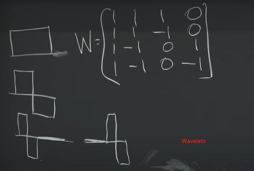
2 Wavelets
- like Handamard Matrix: 1s and -1s (simplest wavlets)
- 下图所示就是一组wavelets
- Haar Wavelets
- W 4 = [ 1 1 1 0 1 1 − 1 0 1 − 1 0 1 1 − 1 0 − 1 ] W_4 = \begin{bmatrix} 1 & 1 & 1 & 0 \\ 1 & 1 & -1 & 0 \\ 1 & -1 & 0 & 1 \\ 1 & -1 & 0 & -1 \end{bmatrix} W4=⎣⎢⎢⎡111111−1−11−100001−1⎦⎥⎥⎤ is a Orthogonal Matrix
- 还可得到8阶
W
8
W_8
W8:
- W 8 = [ 1 1 1 0 1 0 0 0 1 1 1 0 − 1 0 0 0 1 1 − 1 0 0 1 0 0 1 1 − 1 0 0 − 1 0 0 1 − 1 0 1 0 0 1 0 1 − 1 0 1 0 0 − 1 0 1 − 1 0 − 1 0 0 0 1 1 − 1 0 − 1 0 0 0 − 1 ] W_8 = \begin{bmatrix} 1 & 1 & 1 & 0 & 1 & 0 & 0 & 0\\ 1 & 1 & 1 & 0 & -1 & 0 & 0 & 0\\ 1 & 1 & -1 & 0 & 0 & 1 & 0 & 0\\ 1 & 1 & -1 & 0 & 0 & -1 & 0 & 0\\ 1 & -1 & 0 & 1 & 0 & 0 & 1 & 0\\ 1 & -1 & 0 & 1 & 0 & 0 & -1 & 0\\ 1 & -1 & 0 & -1 & 0 & 0 & 0 & 1\\ 1 & -1 & 0 & -1 & 0 & 0 & 0 & -1\\ \end{bmatrix} W8=⎣⎢⎢⎢⎢⎢⎢⎢⎢⎢⎢⎡111111111111−1−1−1−111−1−10000000011−1−11−1000000001−1000000001−1000000001−1⎦⎥⎥⎥⎥⎥⎥⎥⎥⎥⎥⎤
- Note: 归一化需要逐列归一化
- 对 Wavelets 的理解 (以
W
4
W_4
W4为例)
- 第一列:taking the average
- 第二列: taking the differences
- 第三列:taking the differences at a smaller scale
- 第四列:also taking the difference at a smaller scale
- Haar invented this in 1910
- Ingrid Danbechies found a whole lot of families of wavelets that hace good properties in 1988
-
This course:
- About Orthogonal Matrix
- Important orthogonal matrices
- The sources of important orthogonal matrices
Next Course:
- Eigenvectors
- Eigenvalues


 1427
1427


 被折叠的 条评论
为什么被折叠?
被折叠的 条评论
为什么被折叠?
 到【灌水乐园】发言


