Machine Learning-based Selection of Graph Partitioning Strategy Using the Characteristics of Graph D

Machine Learning-based Selection of Graph Partitioning Strategy Using the Characteristics of Graph Data and Algorithm (Regular Papers)的论文介绍

结论：

本篇论文介绍了一种基于机器学习的图分割策略选择算法。该算法通过评估图数据和算法特征，对于给定的图数据，自动确定最优的图分割策略。
其中图分隔策略可参考
算法主要分为两个阶段：特征提取和策略选择。在特征提取阶段，算法将计算图数据中的三种特征：平均度数、连通性和阻碍率。平均度数描述了图的密度，连通性描述了图的联通情况，阻碍率描述了图的难以分割程度。同时，算法还会评估使用不同分割策略的算法特征，包括各种启发式算法的性能和分割结果的质量等。

在策略选择阶段，算法使用机器学习方法来选择最优的图分割策略。算法使用了分类器模型来训练数据，并通过交叉验证来评估不同分类器模型的性能。选择最佳的分类模型后，算法会使用生成的模型对新的图数据进行分类，并选择最优的分割策略。

通过实验评估，该算法在多种复杂图数据上取得了较好的性能，证明了其在实际应用中的可行性和有效性。

ABSTRACT

Analyzing large graph data is an essential part of many modern applications, such as social networks. Due to its large computational complexity, distributed processing is frequently employed. This requires graph data to be divided across nodes, and the choice of partitioning strategy has a great impact on the execution time of the task. Yet, there is no one-size-fits-all partitioning strategy that performs well on arbitrary graph data and algorithms. The performance of a strategy depends on the characteristics of the graph data and algorithms. Moreover, due to the complexity of graph data and algorithms, manually identifying the best
partitioning strategy is also infeasible. In this work, we propose a machine learning-based approach to select the most appropriate partitioning strategy for a given graph and
processing algorithm. Our approach enumerates viable partitioning strategies, predicts the execution time of the target algorithm for each, and selects the partitioning strategy with
the fastest estimated execution time. Our machine learning model is trained on features extracted from graph data and algorithm pseudo-code. We also propose a method that augments real execution logs of graph tasks to create a large synthetic dataset. Evaluation results show that the strategies selected by our approach lead to 1.46× faster execution
time on average compared with the mean execution time of the partitioning strategies and about 0.95× the performance compared to the best partitioning strategy.
AIDB Workshop Reference Format: YoungJoon Park, DongKyu Lee, Tien-Cuong Bui. Machine Learningbased Selection of Graph Partitioning Strategy Using the Characteristics of Graph Data and Algorithm. AIDB 2021.
分析大型图数据是许多现代应用程序的重要部分，例如社交网络。由于其巨大的计算复杂性，通常采用分布式处理。这需要将图数据分布在节点上，而分割策略的选择对任务的执行时间有很大影响。然而，并不存在一个适用于任意图数据和算法的通用分割策略。分割策略的性能取决于图数据和算法的特性。此外，由于图数据和算法的复杂性，手动识别最佳分割策略也是不可行的。在这项工作中，我们提出了一种基于机器学习的方法，为给定的图和处理算法选择最合适的分割策略。我们的方法列举了可行的分割策略，预测了目标算法对每种策略的执行时间，并选择预计执行时间最短的分割策略。我们的机器学习模型是基于从图数据和算法伪代码提取的特征进行训练的。我们还提出了一种方法，增加了图任务的实际执行日志，以创建一个大规模的合成数据集。评估结果表明，我们的方法选定的策略平均执行时间比分割策略的平均执行时间快1.46倍，比最佳分割策略的性能略低0.95倍。

INTRODUCTION

Graph data are prevalent in various fields, such as social networks [41], protein structures [20], web structures [24],textual structures [31], and e-commerce [46]. As the amount of graph data increases fast, distributed computing of graph analysis can be an effective approach for large-scale graph data. For example, it takes more than 10,000 seconds to calculate the local clustering coefficient of each vertex for the Clueweb12 data[4] which has about 6.3 billion vertices and about 66.8 billion edges using 25 machines[21]. There are several kinds of research about distributed graph processing. First, partitioning strategies [38, 6, 15, 49, 43, 33] were proposed to partition graph data into a cluster. Second, distributed graph processing engines [6, 11, 30, 12, 50, 35] emerged to analyze distributed graph data. Finally, parallel
algorithms [22, 16, 28, 29] emerged to exploit the distributed environment. We focus on selecting the best partitioning strategy.
A partitioning strategy determines how vertices and edges are divided into clusters, with the main differentiating points being communication cost, computation time, and replication
factor which means the ratio of the number of the replicated vertex to the number of the original vertex. Existing partitioning strategies can be categorized into model agnostic,
edge-cut partitioning, and vertex-cut partitioning[1], where each may consider locality and/or load-balancing. In this paper, we define a task to be a job that performs a specific
algorithm on a specific graph, and the performance of a partitioning strategy as the execution time of a task under the partitioning strategy after partitioning has finished. The motivation for our research is that the performance of a partitioning strategy is different depending on a task.
Figure 1 represents execution times of some tasks when they are executed with different partitioning strategies. The best partitioning strategy is represented in a dotted bar. The
worst partitioning strategy is represented in a diagonally striped bar. The best partitioning strategy to execute the All-Pair Common Neighborhood (APCN) algorithm for
the Web-Stanford graph data is ‘2D Edge Partition’ partitioning strategy while the worst of it is ‘Hybrid’ in Figure 1a. In cases with different algorithms PageRank and TriangleCount for the same graph data, however, the best strategies are ‘Hybrid’ and ‘Ginger’ respectively, and the
worst strategies are also different in Figure 1b, 1d. In addition, the same algorithm APCN and a different graph data Gemsec-HU show a different performance order also in Figure 1c. The best partitioning strategy for one task can be the worst strategy for another task as seen in Figure 1a, 1b,1c, 1e.
图数据在各个领域都很常见，如社交网络[41]、蛋白质结构[20]、网络结构[24]、文本结构[31]和电子商务[46]。随着图数据量的快速增加，分布式计算图分析可以成为大规模图数据的有效方法。例如，对于有大约63亿个顶点和大约668亿个边的Clueweb12数据[4]，使用25台机器[21]计算每个顶点的局部聚类系数需要超过10,000秒的时间。

有关分布式图处理的研究有几种形式。首先，出现了分割策略[38、6、15、49、43、33]来将图数据分割成一个群集。其次，分布式图处理引擎[6、11、30、12、50、35]出现了，用于分析分布式图数据。最后，出现了并行算法[22、16、28、29]来利用分布式环境。我们关注选择最佳分割策略。
分割策略决定了顶点和边如何划分为簇，主要区别在于通信成本、计算时间和复制因子，即复制顶点数与原始顶点数的比率。现有的分割策略可以分为模型无关、边切割和顶点切割[1]，其中每种策略都可能考虑局部性和/或负载均衡。在本文中，我们将任务定义为在特定图形上执行特定算法的作业，并将分割策略的性能定义为分割完成后在分割策略下任务的执行时间。

我们研究的动机是不同任务的分割策略性能不同。图1表示当它们使用不同的分割策略执行时的某些任务的执行时间。最佳分割策略用虚线表示。最差分割策略用对角线条纹条表示。对于Web-Stanford图像的所有对公共邻居（APCN）算法的最佳分割策略是“2D Edge Partition”分割策略，而Figure 1a中的最差策略是“Hybrid”。然而，在相同的图形数据下使用不同算法的PageRank和TriangleCount的情况下，最佳策略分别为“Hybrid”和“Ginger”，最差策略在Figure 1b、1d中也不同。此外，相同的算法APCN和不同的图数据Gemsec-HU也在图1c中显示出不同的性能顺序。一个任务的最佳分割策略可能是另一个任务的最差策略，如图1a、1b、1c、1e所示。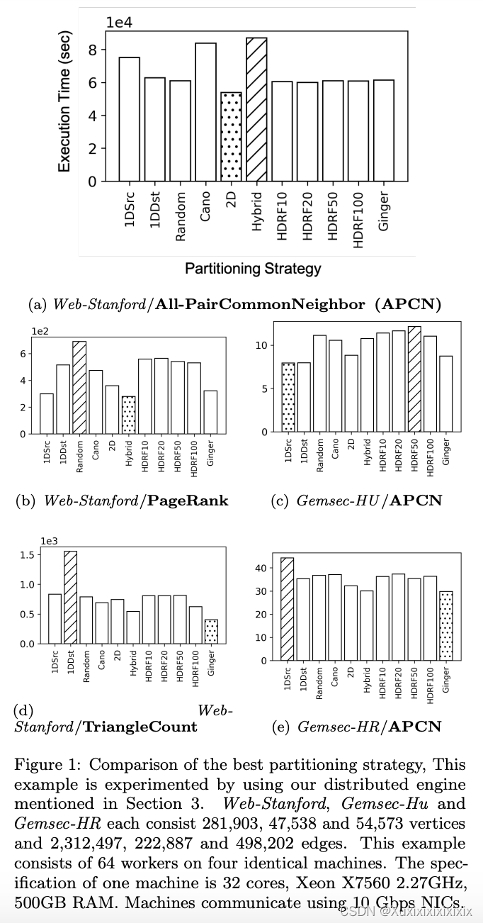
Then, how can we find the most appropriate partitioning strategy that has the best performance for the task? We assume that comprehending the graph data and algorithm can
help select the best partitioning strategy. Several research [45, 36] compare performances of partitioning strategies and propose a decision tree to select the best partitioning strategy. However, they do not declare clear conditions to select decision paths in their decision trees. Also, their heuristic decision trees are not appropriate to cover cases with various
graph data and algorithms. Instead of empirical and heuristic selection of partitioning strategies, we take a machine learning approach that can be generally applied to various
graph data and algorithms. [40, 51] considers graph data to select the best partitioning strategy. They chose only one algorithm, PageRank, to compare the performance of partitioning strategies and did not consider algorithm characteristics. We instead extract graph data and algorithms’ features by carefully analyzing execution behaviors. By that, our method proposes the most suitable strategy to divide data across workers. Figure 2-○1 ,
○2 shows extracting the
features of the task. The task feature is the concatenation
of graph data statistics and algorithm execution pattern
features. Figure 2-○3 shows predicting the performance for
each partitioning strategy using the task feature. We used a
machine learning technique in this part, and our approach
is similar to the concept of software 2.0 supporting systems
using data-driven methods. There are research papers related to database configuration tuning [52, 44], relational
table partitioning [14] and cardinality estimation [47]. We
select the strategy with the fastest expected execution time
in Figure 2-○4 . Figure 2-○5 depicts the training process of
the Execution Time Regression Model (ETRM). We use the
augmented synthetic training dataset as the execution logs
and train the model using the loss between these logs and
the model’s outputs.
We encounter several challenges in designing and implementing the proposed model. First, we have to predict the
execution time of a task by extracting its features without
actually performing it. Next, we need to carefully analyze
both algorithms and graph data to extract useful features
that can be used for the strategy selection model. In addition, we need a large dataset to train the machine learning model. Creating a sufficient real execution log for the training dataset consumes much computing power, so we construct a synthetic training dataset by augmenting real execution logs. Finally, excluding some characteristics of several distributed graph engines, we have to implement an experimental distributed graph engine which the all graph algorithms run on and which covers various partitioning strategies.
We performed several experiments, and a list of experiments is as follows. i) How well our model can select the best partitioning strategy for test cases, ii) how superior the selected strategy’s performance is compared to other strategies, and iii) how much performance benefit our approach can get. The main contributions of our research are the following:
∙ We propose a method to choose the best partitioning strategy using extracted features from graph data and algorithms.
∙ We construct an experimental distributed graph engine, so only the factors for graph data, algorithm, and partitioning strategy be the experimental elements.
∙ We propose a method to generate synthetic training data to train our model. The rest of this paper is organized as follows. In Section 2, we summarize notations. In Section 3, we describe our distributed graph computation engine that we implemented for experimental purposes. In Section 4, we describe the set of features we extracted and how. In Section 5, we evaluate our method. In Section 6, we review related works. We conclude and propose future work in section 7.
我们在设计和实施所提出的模型时遇到了几个挑战。首先，我们需要提取任务的特征以预测其执行时间，而不实际执行它。接下来，我们需要仔细分析算法和图形数据以提取可用于策略选择模型的有用特征。此外，我们需要一个大型数据集来训练机器学习模型。创建足够的实际执行日志用于训练数据集会消耗大量计算能力，因此我们通过增加实际执行日志来构建一个合成的训练数据集。最后，除了几个分布式图形引擎的某些特征之外，我们还必须实现一个实验性的分布式图形引擎，在其中所有图形算法都运行，并涵盖各种分区策略。

我们进行了几项实验，实验包括：i）我们的模型可以为测试用例选择最佳分区策略多好。ii）所选策略的性能与其他策略相比有多超越。iii）我们的方法可以获得多少性能提升。

我们的研究的主要贡献如下：

∙ 我们提出了一种使用从图形数据和算法中提取的特征选择最佳分区策略的方法。

∙ 我们构建了一个实验性分布式图形计算引擎，使图形数据、算法和分区策略成为实验元素。

∙ 我们提出了一种生成合成训练数据来训练我们的模型的方法。

本文的其余部分如下：在第2节中，我们总结符号。在第3节中，我们描述了我们实施的分布式图计算引擎。在第4节中，我们描述了我们提取的一组特征以及如何提取特征。在第5节中，我们评估了我们的方法。在第6节中，我们回顾了相关工作。我们在第7节中总结并提出了未来的工作。

NOTATIONS

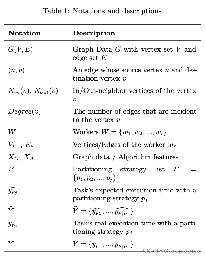
We summarize notations used in this paper in Table 1. These notations include the vertex set 𝑉 , edge set 𝐸, and neighbor vertex 𝑁(𝑢) related to the graph data 𝐺. In addition, Table 1 includes the worker set 𝑊, the partitioned vertex set and edge set used in distributed processing, and the notations used in the execution time regression model.

3. DISTRIBUTED GRAPH ENGINE

This section describes our graph computation engine, which serves as a test bed for comparing the partitioning strategy execution process. This paper focused on the partitioning
strategies related to the data and the algorithm. Therefore, our graph engine contains essential functions and operators that serve our purpose.

3.1 Graph Representation

As we focused only on the task’s performance, we simplified the implementation. Our graph engine used an edge list to represent the graph data. The edge list consists of vertex tuples, (𝑢, 𝑣). An inverted edge list is also maintained. Finding a vertex takes 𝑂(𝑙𝑜𝑔(|𝑉 |)) time. It takes 𝑂(𝑑𝑒𝑔𝑟𝑒𝑒(𝑣)) to search for an edge connected to an arbitrary vertex 𝑣 by managing a key-value hash map with vertex id as a key and the starting point of the edge list connected to this vertex as value. The edge list is sorted by source vertex ID. Thus, insertion and deletion are also ignored. In addition, vertex and edge properties are stored in each key-value map.

3.2 Distributed Computation Model

3.2.1 GAS Model for Distributed Computing

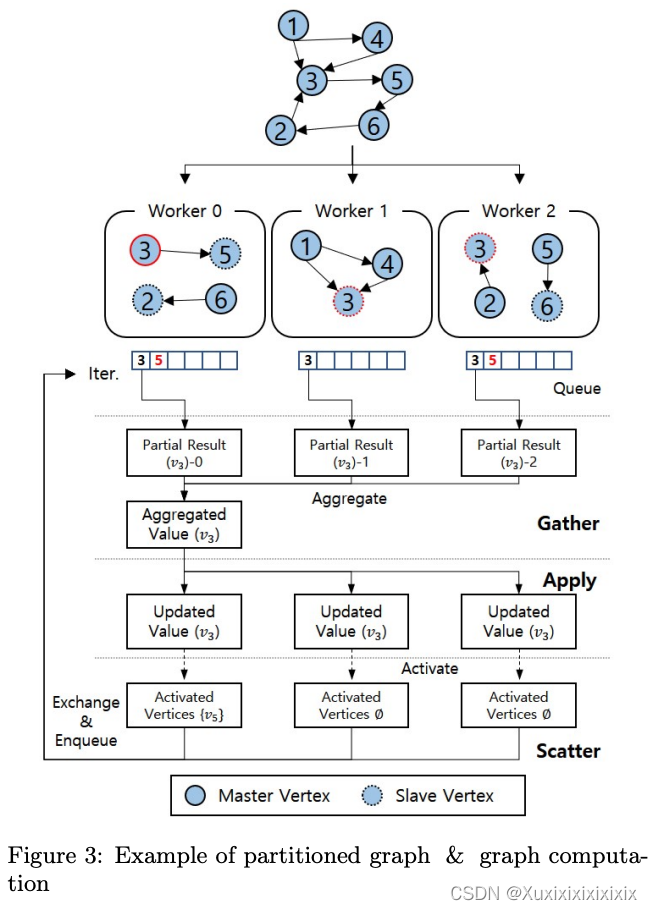
Among several distributed graph computation models, we selected the GAS model[11]. Hadoop MapReduce[42] is general and can be used in various applications, but is not suitable because it uses HDFS[3], which can cause excessive I/O and it may run unnecessary shuffle operations. TUX2 [48]proposed the MEGA model, which is optimized for graph machine learning algorithms. We didn’t adopt the MEGA model because we target more general graph processing tasks instead of specific graph ML tasks The GAS model is a vertex-centric model[32] and ‘GAS’ stands for Gather, Apply and Scatter. While partitioning edges separately, vertices that exist commonly in partitioned edges are replicated. The GAS model sets one vertex as the master vertex and the others as mirror vertices with the same vertex ID vertices. Workers have a queue for representing vertices that will be processed locally. Each
worker pops a vertex from the queue and propagates it to the corresponding workers having mirror vertices. For each of these vertices in the Gather phase, the engine collects all
mirrors’ local results and aggregates them. In the Apply phase, the master vertex’s aggregated result is transmitted to mirror vertices. In the Scatter phase, the vertex’s aggregated result is used to update its adjacent edges. The neighbor vertices are enqueued if these neighbor vertices are needed to be computed. This activation occurs based on the local
neighbor, and this result is shared between workers. Vertex 3’s GAS step is illustrated in Figure 3. In this example, 𝑣3’s partial result is computed in each worker and aggregated to
worker 0. Then, this aggregated value is updated to mirror vertices. Lastly, in this example, out-neighbor 𝑣5 is activated and en-queued.

3.2.2 Scalability

We tested the scalability of our engine to show that theimplementation is scalable enough to conduct our experiments. This result can be seen in Figure 4. This experiment consisted of 4, 8, 16, 32, and 64 workers on four identical machines. The specification of one machine is 32 cores, Xeon X7560 2.27GHz, 500GB RAM. Machines communicate using 10 Gbps NICs. PageRank and TriangleCount algorithms were performed for Web-Stanford data. We could see that execution time decreased for two algorithms up to 64 workers.
本节描述了我们的图形计算引擎，它作为比较分区策略执行过程的测试平台。本文重点关注与数据和算法相关的分区策略。因此，我们的图形引擎包含为此目的服务的基本功能和运算符。

3.1 图表示方法

由于我们只关注任务的性能，我们简化了实现。我们的图形引擎使用边列表表示图形数据。边列表由顶点元组(𝑢，𝑣)组成。还维护了一个反向边列表。查找顶点需要𝑂(𝑙𝑜𝑔(|𝑉|))的时间。通过使用顶点ID作为键，连接到该顶点的边列表的起始点作为值，通过管理键值哈希映射查找连接到任意顶点𝑣的边需要𝑂(𝑑𝑒𝑔𝑟𝑒𝑒(𝑣))时间。边列表按照源顶点ID排序。因此，插入和删除也被忽略。此外，每个键值映射中存储顶点和边的属性。

3.2 分布式计算模型

3.2.1 基于GAS模型的分布式计算

在几种分布式图计算模型中，我们选择了GAS模型[11]。Hadoop MapReduce[42]是通用的，可以用于各种应用程序，但不适合我们的使用场景，因为它使用HDFS[3]，可能会导致过多的I/O和不必要的洗牌操作。TUX2 [48] 提出了MEGA模型，该模型针对图形机器学习算法进行了优化。我们没有采用MEGA模型，因为我们的目标是更通用的图形处理任务，而不是特定的图形机器学习任务。GAS模型是一个以顶点为中心的模型[32]，‘GAS’代表“We Gather, We Apply, We Scatter”（我们收集、我们应用、我们散布）。在单独分区边的同时，存在于分区边中的顶点是复制的。GAS模型将一个顶点设置为主节点，其他顶点作为具有相同顶点ID的镜像顶点。工作者维护一个队列，用于表示将在本地处理的顶点。每个工作者从队列中弹出一个顶点并将其传播到具有镜像顶点的相应工作者。在聚集阶段，对于每个镜像顶点，引擎收集所有镜像的本地结果并进行聚合。在应用阶段，将主节点的聚合结果传输到镜像顶点。在散布阶段，使用顶点的聚合结果更新其相邻边。如果需要计算这些相邻顶点，则将这些相邻顶点入队。这个激活是基于本地相邻节点完成的，并且此结果在工作者之间共享。图3描绘了顶点3的GAS步骤。在这个例子中，𝑣3的部分结果在每个工作者中计算并聚合到工作者0中。然后，将该聚合值更新到镜像顶点。最后，在这个例子中，出邻居𝑣5被激活并入队。

3.3 Partitioning Method
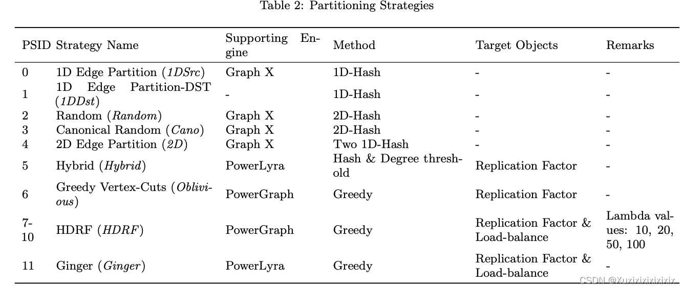
The partitioning methods used in our test bed were selected based on the following criteria: i) commonly used in many systems, and ii) proper to processing model. We selected GAS as the distributed graph processing model, and accordingly, we employed partitioning methods supported by representative GAS systems such as GraphX, PowerGraph, and PowerLyra. The following describes the partitioning methods supported by our engine. Table 2 shows a brief summary of each partitioning strategy.

3.3 分区方法

我们在测试平台中选择的分区方法基于以下标准：i）在许多系统中常见，ii）适合处理模型。我们选择了GAS作为分布式图处理模型，因此，我们采用了代表性GAS系统如GraphX、PowerGraph和PowerLyra支持的分区方法。以下描述了我们的引擎支持的分区方法。表2显示了每个分区策略的简要总结。

4. STATIC ANALYSIS AND EVALUATION

To prove our hypothesis that we can choose a better partitioning strategy by analyzing the data and the algorithm, we extracted certain features. The structural properties of graph data are summarized by statistic values, and symbolic code analysis on the pseudo-code of the algorithm is conducted to get the algorithm features. Finally, a machine learning model is constructed to predict how long does it take for given tasks. The overall process can be seen in Figure 2. Section 4.1 explains how the features are extracted from the graph data and algorithm. Section 4.2 explains the Execution Time Regression Model that predicts the performance of partitioning strategy using machine learning.

4.1 Feature Extractor

4.1.1 Data Feature

Various inherent features in the graph data were selected for the following reasons and summarized in Table 3.The number of vertices and edges is helpful in analyzing the iteration over the entire graph and predicting the iteration’s execution time. Graph data always represent the relationship between vertices as edges, and graph data analysis commonly accompanies access to edges. Therefore, it is necessary to understand the graph topology because the degree of vertices and their distribution vary according to the topology. We extracted mean, standard deviation, skewness, and kurtosis from each vertices’ in-degree and out-degree. Since skewness and kurtosis can have negative values, they are divided into a sign and absolute value and used as input features. Furthermore, it is essential to consider whether the graph is directed because some operators behave differently (e.g. get in-neighbors of some vertex, inverted edge list).

4.1.2 Algorithm Feature

The frequency of graph operations are evaluated to capture the pattern and scale of data access for executing the graph algorithm. We wrote a code analyzer with JavaCC, a compiler-compiler tool like YACC. It analyzes the pseudocode which consists of graph operators supported by our engine. The operators are listed in Table 4. The pseudo-code has symbols representing graph elements such as ALL VERTEX LIST, GET IN VERTEX TO as seen in Listing 1. Parsing the code, the number of each graph and arithmetic operation is counted. As a result, the key-value pairs as operation-count will be generated as seen in line 1 of Listing 2. Even if it cannot be evaluated as a real value, the count is represented by a symbolic expression. In order to fill in those symbols with real values, data features are used to evaluate the symbols. For example, a graph operation GET IN VERTEX TO(v) in line 10 of Listing 1 is found at the condition of for loop in line 10. The number of this operation
can be evaluated by the multiplication of outer loop variables, |ALL VERTEX LIST|*iterator num. The number of iteration can be found in line 1 of Listing 1, so it is immediately evaluated as 20.0. The size of all vertex set is trivially same as |𝑉 |, the cardinality of the vertex set of graph. Thus, the number of all vertex can be taken from data feature 𝐷𝐹. The graph data in this example was Ego-Facebook[25] and |𝑉 | is 4039 so, the final counting value of GET IN VERTEX TO becomes 4039 * 20.0 = 80780.0. The accesses to variables and arithmetic operators are also counted to precisely

4.2 Execution Time Regression Model

We implemented a prediction model to select the best partitioning strategy in a given task. We tried some machine learning models such as linear regression, XGBoost[7], LightGBM[20], multi-layer perceptron and mixture of experts [17]. The best model was the XGBoost regression model.The training process and model structure of the Execution Time Regression Model are as follows.

4.2.1 Data Preparation

We executed tasks encompassing the graph data, algorithms, and partitioning strategies on our engine and recorded execution logs. The graph data and algorithm in the execution log are mapped to the data feature and the algorithm feature respectively by the feature extractor. We prepared total execution logs using 12 graph data, 8 algorithms, and 11 partitioning strategies except Oblivious strategy. To train our machine learning model, we had to prepare a
huge amount of training set. Among those execution logs, 528 logs made by 8 graph data, 6 algorithms, and 11 partitioning strategies were used to create the augmented training dataset.
We generated synthetic data via aggregation of multiple real data records. Aggregation is the summation of the algorithm feature and execution time by grouping the logs performed
in the same graph data with the same partitioning strategy. The task of a synthetic tuple is interpreted as one large algorithm with several algorithms performed sequentially.
Therefore, the algorithm features that predict the number of calls for the low-level function and the execution time can be aggregated by summation. For example, if a synthetic tuple
𝑠 is created via aggregation of real tuples 𝑟1, 𝑟2, …, 𝑟𝑛, then tuple 𝑠’s algorithm feature is 𝐴𝐹(𝑠) = ∑︀𝑛𝑖 𝐴𝐹(𝑟𝑖). It’s data feature is 𝐷𝐹(𝑠) = 𝐷𝐹(𝑟1) = … = 𝐷𝐹(𝑟𝑛) and execution
time is 𝐸𝑇(𝑠) = ∑︀𝑛 𝑖 𝐸𝑇(𝑟𝑖).We used combinations with replacement to make the synthetic algorithms. The formula is as follows.
𝐶
𝑅
(𝑛, 𝑟) = (𝑛 + 𝑟 − 1)!
𝑟!(𝑛 − 1)! (3)
We created synthetic algorithms by using 6 original algorithms and changing r from 2 to 9. The number of synthetic algorithms is ∑︀9𝑟=2 𝐶𝑅(6, 𝑟) = 4998. Our synthetic training dataset has about 0.43 million tuples by multiplying 4998 synthetic algorithms, 8 graph data and 11 partitioning strategies. Since each sample of the synthetic dataset has a different combination of algorithms, the entire synthetic dataset can be interpreted as a record of performing various and unique algorithms. The augmented training dataset does not include the original 528 real records. We used 528 records and records from other 4 graph data and 2 algorithms in the test phase.

4.2.2 Model Architecture

Our model captures the features of data and an algorithm to predict their execution time of a task for a given partitioning strategy. XGBoost regression model includes regularization term and uses Classification And Regression Tree (CART) ensemble model. This ensemble model decides whether to split the branch to maximize the Gain and minimize the Objective function. The formula is as follows.
𝑦ˆ𝑖
(𝑡) = prediction of the i-th instance at the t-th iteration
(4)(5) (6) (7)
𝐼𝐿 = the instance sets of left node after the split (8) 𝐼𝑅 = the instance sets of right node after the split (9)
𝐼 = 𝐼𝐿 ∪ 𝐼𝑅 (10)
𝜆 = L2 regularization term on weights (11)
𝛾 =
minimum loss reduction required to make a
further partition on a leaf node of the tree (12)
𝐺𝑎𝑖𝑛 (13)
Ω = regularization term (14)
𝑓𝑘 = k-th decision tree in function space F (15)
𝑜𝑏𝑗𝑒𝑐𝑡𝑖𝑣𝑒 =|𝑆𝑎𝑚𝑝𝑙𝑒𝑠∑︁|𝑖=1𝑙𝑜𝑠𝑠(𝑦𝑖, 𝑦ˆ𝑖(𝑡−1)) +∑︁𝐾𝑘=1Ω(𝑓𝑘) (16)
We used the XGBRegressor model and the detailed parameters of the Regressor are as follows.
∙ colsample bytree = 0.4603
∙ gamma = 0.0468
∙ learning rate = 0.05
∙ max depth = 15
∙ min child weight = 1.7817
∙ n estimators = 1000
∙ reg alpha = 0.4640
∙ reg lambda = 0.8571
∙ subsample = 0.5213
∙ objective = squared error
The input of the model is expressed as 𝑋. 𝑋 has both graph data features 𝑋𝐺 and algorithm features 𝑋𝐴 pre-processed with scaling and one-hot encoding. Figure 5 describes the model’s input data.

4.静态分析与评估

为了证明我们能通过分析数据和算法选择更好的分区策略的假设，我们提取了一些特征。图数据的结构性质由统计值进行总结，对算法伪代码进行符号代码分析以获得算法特征。最后，构建机器学习模型以预测给定任务所需时间。整个过程如图2所示。第4.1节解释了如何从图数据和算法中提取特征。第4.2节解释了执行时间回归模型，该模型使用机器学习预测分区策略的性能。 图数据中的各种固有特征被选择出来，原因如下，并在表3中总结。顶点和边的数量有助于分析整个图的迭代，并预测迭代的执行时间。
图形数据始终将顶点之间的关系表示为边，并且图形数据分析通常需要访问边。因此，了解图形拓扑结构是必要的，因为顶点的度数和其分布会根据拓扑结构而变化。我们从每个顶点的入度和出度中提取均值、标准差、偏度和峰度。由于偏度和峰度可能具有负值，因此它们被分为符号和绝对值，并用作输入特征。
此外，考虑图形是否为有向图形也是必要的，因为一些运算符的行为不同。

4.1.2 算法特征

对图操作的频率进行评估，以捕捉执行图算法时的数据访问模式和规模。我们使用JavaCC编写了一个代码分析器，它是一种类似于YACC的编译器编译器工具。它分析了由我们的引擎支持的图操作组成的伪代码。这些操作列在表4中。
该伪代码具有代表图元素的符号，例如在清单1中看到的ALL VERTEX LIST、GET IN VERTEX TO等。解析代码时，每个图和算术运算的数量都会被计算。因此，键值对作为操作计数将生成，如清单2的第1行所示。即使它不能被评估为实际值，计数也用符号表达式表示。为了用实际值填充这些符号，使用数据特征来评估符号。例如，在清单1的第10行找到的图操作GET IN VERTEX TO(v)在循环的条件中发现。此操作的数量可以通过外部循环变量|ALL VERTEX LIST|*iterator num的乘法来评估。迭代次数可以在清单1的第1行找到，因此它立即评估为20.0。所有顶点集的大小与图的顶点集的势𝑉 的基数显然相同。因此，所有顶点的数量可以从数据特征𝐷𝐹中获得。
此示例中的图形数据是Ego-Facebook[25]，|𝑉 |为4039，因此GET IN VERTEX TO的最终计数值为4039 * 20.0 = 80780.0。
还会计算对变量和算术运算符的访问，以精确评估循环体即清单2的第5、12行。

4.2 执行时间回归模型

我们实现了一个预测模型来选择给定任务中的最佳分区策略。我们尝试了一些机器学习模型，如线性回归、XGBoost[7]、LightGBM[20]、多层感知器和专家混合[17]。最佳模型是XGBoost回归模型。
执行时间回归模型的训练过程和模型结构如下。

4.2.1 数据准备

我们在我们的引擎上执行图数据、算法和分区策略涉及的任务，并记录执行日志。执行日志中的图数据和算法分别由特征提取器映射到数据特征和算法特征上。我们使用了12个图形数据、8个算法和11个分区策略（不包括Oblivious策略）来准备总执行日志。
为了训练我们的机器学习模型，我们必须准备大量的训练集。其中，使用了由8个图形数据、6个算法和11个分区策略生成的528个日志，以创建增广的训练数据集。我们通过聚合多个真实数据记录生成合成数据。聚合是通过将在相同图形数据和分区策略下执行的日志分组并进行算法特征和执行时间的总和来实现的。
合成元组的任务被解释为一个大算法，其中包含按顺序执行的多个算法。因此，可以通过求和来聚合用于预测低级函数调用次数和执行时间的算法特征。例如，如果通过汇总真实元组𝑟1、𝑟2、…、𝑟𝑛创建了合成元组𝑠，则元组𝑠的算法特征为𝐴𝐹(𝑠)=∑︀𝑛
𝑖 𝐴𝐹(𝑟𝑖)。其数据特征为𝐷𝐹(𝑠)=𝐷𝐹(𝑟1)=…=𝐷𝐹(𝑟𝑛)，执行时间为𝐸𝑇(𝑠)=∑︀𝑛
𝑖 𝐸𝑇(𝑟𝑖)。
我们使用重复组合来生成合成算法。公式如下。
𝐶
𝑅
(𝑛, 𝑟) = (𝑛+𝑟−1)!
𝑟!(𝑛−1)! (3)
我们使用6个原始算法，将r从2更改为9来创建合成算法。共创建了4998个合成算法。我们的合成训练数据集大约有430,000个元组，通过乘以4998个合成算法、8个图形数据和11个分区策略来实现。由于合成数据集的每个样本都具有不同的算法组合，整个合成数据集可以被解释为执行各种独特算法的记录。增广的训练数据集不包括原始的528条真实记录。我们在测试阶段使用了528条记录以及其他4个图形数据和2个算法的记录。
… … …
后续参考原文即可
原文链接