Bayesian framework 贝叶斯框架 （R）

写在前面

本文介绍了 Bayes' theorem（贝叶斯定理），Bayesian inference（贝叶斯推理），Bayesian regression Model （贝叶斯回归模型） 等。

贝叶斯定理大家都耳熟能详，高中数学甚至都有涉及，即：用先验概率和条件概率求出另外的条件概率。

但贝叶斯推理和回归模型我认为是一个比较trick 的内容。

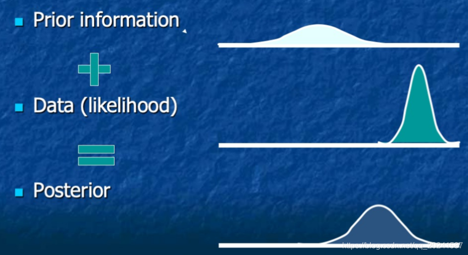
用一张图解释本文的内容：

一些术语

prior :   1 happening or existing before sth else or before a particular time  ,  2 already existing and therefore more important；

likelihood : 参考我之前的博客；

posterior : located behind sth or at the back of sth

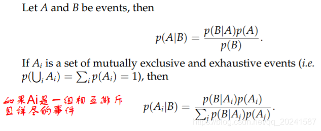
Bayes' theorem 贝叶斯定理

简单来说就是用先验概率和条件概率求出另外的条件概率。

Bayesian inference

将贝叶斯定理应用在统计分析中, 即模型参数是未知量, 而且它们的先验分布需要被（手动/经验地）指定 — this is Bayesian inference.

（在贝叶斯框架中，我们讨论的是模型参数的概率分布 ，注意，在那些常见的框架中，如以MLE为基础的GLM，模型参数是 fixed non-random quantities ，数据才是遵循某种概率分布 ，这是两者显著的不同。

一个粗鲁的解释就是：我们有一堆观测数据，我们揣测这个数据可能符合某种模型分布，如正态。泊松等，然后模型的参数也被我们 揣测地 定了下来， 然后我们用观测数据和这个我们揣测的模型 去收敛训练， 最后我们得到了 posterior ，这个 posterior，是 我们根据观测数据收敛训练，得到的模型的参数 ，注意我们得到的是参数的分布，而不是点估计。

 

更多的可以参考这里。）

假设：

1 观测量，即数据 ，是 x；

2 位置量是θ，这个 θ 可以代表模型参数，数据中地缺失值，误测值等；

基于我们上面的假设，

首先我们提出 likelihood ：p(x | θ)

然后我们从贝叶斯定理的角度观察 ： θ 是未知的，所以它需要有（被手动/经验地指定）一个概率分布，用来表示这个 不确定性； x 是已知的，所以它是条件（condition on it），我们得到 posterior distribution ：

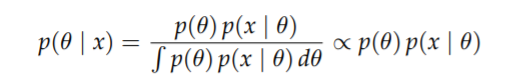
所以总的来说，我们首先指定了一个  prior distribution p(θ), 表达了我们在看到数据之前对θ不确定性的预估. The posterior distribution p(θ | x), 表达了我们在看到数据之后对θ不确定性的预估。

很明显：1 我们的 posterior 是prior 和 data （likelihood） 的居中选择，2 如果我们的数据越多，我们的 data （likelihood ）的 影响力就越大，prior 影响力就越小 （比如你认为 它们都是好的，但搞了一堆观测数据发现它们基本都是坏的，那推论 必然更容易是 它们是坏的）

 

MCMC Markov chain Monte Carlo 马尔可夫链蒙特卡洛

既然我们手工地指定了模型参数 prior ，那怎么具体的通过数据 data （likelihood），得到后验posterior 呢？

（显然这里和以前的GLM/LM不同，这个方法对prior的依赖是显而易见的，而线性模型中我们更希望贴近数据，模型参数的初值完全是random设定的，最终收敛得到的参数完全由最优化损失函数/或MLE决定，而在这里我们极大程度上的参考了prior的意见 ，而且 以前我们是考虑模型参数的点估计，这里我们是得到模型参数的概率分布， 这就是这两个方法显而易见的差别。）

 MCMC 是解决上诉问题的一个方法：

We have already seen that Monte Carlo methods can be used to simulate values from prior distributions and from closed form posterior distributions If we had algorithms for sampling from arbitrary (typically high-dimensional) posterior distributions, we could use Monte Carlo methods for Bayesian estimation:

这方法具体的数学实现我就不说了，没这能力......但给个代码的例子还是OK的。

创建一个具有期望属性的马氏链并非难事，难的是如何决定通过多少步可以达到在许可误差内的稳定分布。一个好的马氏链具有快速混合——从开始阶段迅速获得的一个稳定状态。

Bayesian regression models

标准(和非标准)回归模型可以很容易地在贝叶斯框架内建立。

• Specify probability distribution (likelihood) for the data
• Specify form of relationship between response and explanatory variables 明确预测与响应变量之间的关系
• Specify prior distributions for regression coefficients and any other unknown (nuisance) parameters 指定模型系数的 prior

Bayesian Linear regression

注意这里我们给出了一个较为通用的prior，当然这东西是非常vague的，视情况而定

 

 

 

 

一个R的例子

这是一个贝叶斯线性回归模型，包括它的建模和一些推论

#工会密度被定义为属于工会的劳动力的百分比。
#关于如何解释工会密度的跨国变化，有许多相互矛盾的理论。

#为了探索不同的理论，我们使用了n = 20个自二战以来有着连续民主历史的国家的数据。
#我们有以下变量:工会密度(Uden)，劳动力规模(LabF)，工业集中度(IndC)，
#左翼政府(LeftG)，测量于20世纪70年代末
#We fit the following linear regression model:
#                Udeni ∼ N(µi, σ2)
#     µi = b0 + b1(LeftGi − LeftG) + b2(LabFi − LabF) + b3(IndCi − IndC)
#with vague priors
#     1/σ2 ∼ Gamma(0.001, 0.001)
#     b0 ∼ N(0, 100000)
#     b1 ∼ N(0, 100000)
#     b2 ∼ N(0, 100000)
#     b3 ∼ N(0, 100000)
#在union-dat文件中提供了假设每个回归系数具有模糊先验的数据、
#一些初值和基本模型文件。odc, union-in1。odc, union-in2。odc union-model.odc。
#注意，本例中的数据是“矩形数组”数据格式，而不是“列表”格式。
#20行对应国家，列分别给出4个变量(response和3个predictors)。
#要将这些数据加载到WinBUGS中，突出显示包含列名的第一行，
#并在适当的阶段单击load data(如果数据文件是焦点窗口，
#                   只需单击load data而不突出显示第一行也可以)。


library(R2jags)
library(coda)
library(lattice)
#Next we define the model. We have observations from 20 countries, hence the for loop. Note that for logical
#nodes (that is when the variable can be defined using < −) we can take advantage of the vectorised way R
#does computations, but in case of stochastic dependence (when we are using ∼) we have to use a for loop.
#接下来定义模型。我们有来自20个国家的观察结果，因此有for循环。请注意，对于逻辑节点(即可以使用<−定义变量)，
#我们可以利用向量化的方式R进行计算，但是对于随机相关(当我们使用∼)，我们必须使用for循环。
jags.mod <- function(){
  for(i in 1:20){
    Uden[i]~dnorm(mu[i],tau) # normal likelihood
    # linear predictor with centered covariates
    mu[i] <- b0+b[1]*(LeftG[i]-mean(LeftG[]))+
      b[2]*(LabF[i]-mean(LabF[]))+b[3]*(IndC[i]-mean(IndC[]))
  }
  # prior on residual error variance
  tau ~ dgamma(0.001,0.001)
  sigma2 <- 1/tau # residual error variance
  # vagues priors on regression coefficients
  b0 ~ dnorm(0,0.00001)
  for(k in 1:3){
    b[k] ~ dnorm(0,0.00001)
  }
}
dat <- c(82.4,8.28,111.84,1.55,80.0,6.90,73.17,1.71,
         74.2,4.39,17.25,2.06,73.3,7.62,59.33,1.56,
         71.9,8.12,43.25,1.52,69.8,7.71,90.24,1.52,
         68.1,6.79,0.00,1.75,65.6,7.81,48.67,1.53,
         59.4,6.96,60.00,1.64,58.9,7.41,83.08,1.58,
         51.4,8.60,33.74,1.37,50.6,9.67,0.00,0.86,
         48.0,10.16,43.67,1.13,39.6,10.04,35.33,0.92,
         37.7,8.41,31.50,1.25,35.4,7.81,11.87,1.68,
         31.2,9.26,0.00,1.35,31.0,10.59,1.92,1.11,
         28.2,9.84,8.67,0.95,24.5,11.44,0.00,1.00)

dat <-matrix(dat,nrow=20,ncol=4,byrow=TRUE)
Uden <- dat[,1]
LabF <- dat[,2]
LeftG <- dat[,3]
IndC <- dat[,4]
jags.data <- list("Uden","LabF","LeftG","IndC")

#Set the parameters we want to monitor. At this stage these are the regression coefficients.
# Parameters we want to monitor
# Same as "set"ting these variables in WinBUGS
jags.param <- c("b0","b")
#Specify initial values. To check convergence we are planning to run 2 chains, 
#thus we need two sets of initial values for the random parameters. 
#These again should be passed on as a list. Note that Gelman-Rubin convergence diagnostic 
#is not possible with a single chain.
#指定初始值。为了检查收敛性，我们计划运行2个链，因此我们需要为随机参数设置两组初始值。
#这些应该作为列表传递。请注意，盖尔曼-鲁宾收敛诊断是不可能与一个单一的链。
# Specify initial values
inits1 <- list("tau" = 100, "b0" = 20, "b"=c(10,-5,-25))
inits2 <- list("tau"=100000,"b0"=-100,"b"=c(-100,100,500))
jags.inits <- list(inits1, inits2)

#Fit the model. We set the number of chains to two, draw 6000 samples for each chain, 
#but discard the first 1000 samples as burn-in. 
#At this stage we don’t want to thin the samples 
#(we can run the model again if the autocorrelation plots reveal correlation between samples),
#so we set n.thin to 1.
#合适的模型。我们设置了两个链的数量，每个链抽取6000个样本，但丢弃前1000个样本作为老化。
#在这个阶段，我们不想细化样本(如果自相关图显示样本之间的相关性，我们可以再次运行模型)，
#所以我们设置n.thin to 1。
# Fit the JAGS model
jags.mod.fit <- jags(data = jags.data, inits = jags.inits,
                     parameters.to.save = jags.param, n.chains = 2, n.iter = 6000,
                     n.burnin = 1000,n.thin=1,model.file = jags.mod)
#这为我们提供了监测后节的简要统计(平均值、sd、分位数)。
#此外，还给出了收敛性和有效样本容量的一些信息，
#这些信息可以帮助我们判断样本之间是否存在相关性。
print(jags.mod.fit)
#然而，为了收敛，最好是提取G-R测试统计量，一旦拟合的模型转换成一个MCMC对象:
jagsfit.mcmc <- as.mcmc(jags.mod.fit)
gelman.diag(jagsfit.mcmc)
#如果链已经收敛，这些值应该接近1(任何大于1.1的值通常表示缺乏收敛性)。
#如果>。diag命令不运行，请尝试将多元参数设置为FALSE。
#这里我们有完美的收敛，如果没有收敛，我们可以绘制新的样本使用'更新'函数:
jags.mod.fit.upd <- update(jags.mod.fit, n.iter=10000)
# Look at the outcome
print(jags.mod.fit.upd)
#用中位数绘制80%的intervals，作为posteriors
plot(jags.mod.fit)
#我们可以通过导出来自jags结果的样本来分别查看箱线图。
#模拟样本在jags.mod.fit$BUGSoutput$sims中。对象列表。
# boxplot
beta <- as.data.frame(jags.mod.fit$BUGSoutput$sims.list$b)
colnames(beta) <- c("b1","b2","b3")
boxplot(beta,outline=FALSE)
#the extracted samples we can also produce scatter plots to assess 
#whether there’s correlation between the different coefficients
#提取的样本也可以制作散点图来评估不同系数之间是否存在相关性
plot(beta$b1,beta$b2,xlim=c(-0.2,0.6),ylim=c(-40,20))
plot(beta$b2,beta$b3,xlim=c(-40,20),ylim=c(-100,100))
plot(beta$b3,beta$b1,ylim=c(-0.2,0.6),xlim=c(-100,100))
#can look at the trace plots, or use the mcmc object for more summaries, plots. 
#Since we specified the burn-in at the start these samples are not 
#included in the summary statistics.
#可以查看跟踪图，或使用mcmc对象获取更多摘要、图。
#由于我们在开始时指定了老化，所以这些样本不包括在汇总统计数据中。
traceplot(jags.mod.fit)
# Convert into an MCMC object for more diagnostics 转换成MCMC对象以进行更多的诊断
jagsfit.mcmc <- as.mcmc(jags.mod.fit)
summary(jagsfit.mcmc)
plot(jagsfit.mcmc)
xyplot(jagsfit.mcmc)
densityplot(jagsfit.mcmc)
#Using the autocorr.plot function we can assess
#whether there’s autocorrelation between the samples. 
#Ideally we want to get 1 at lag = 0, and values close to 0 afterward.
#If the values are quite high up to lag = k, 
#then the problem of correlated samples can be resolved
#by setting n.thin=k+1 when we are fitting the model.
#使用autocorr.plot function我们可以评估样本之间是否存在自相关
#理想情况下，我们希望get 1 at lag = 0，之后得到接近0的值
autocorr.plot(jagsfit.mcmc)
#Here we shouldn’t worry about autocorrelation too much. There might be a slight correlation at lag=1 for
#b[1], but it’s not very strong, so here we won’t do any thinning. To get rid of that possible correlation you
#can set n.thin=2 when you’re fitting the model. Note however that that will halve your obtained samples
#To get boxplots for the mean union density we have to add mu to the list of monitored parameters, then fit
#the model again
jags.param <- c("mu","b0","b")
jags.mod.fit <- jags(data = jags.data, inits = jags.inits,
                     parameters.to.save = jags.param, n.chains = 2, n.iter = 6000,
                     n.burnin = 1000,n.thin=1,model.file = jags.mod)
# Boxplots where the means are ordered according to their median
mu <- as.data.frame(jags.mod.fit$BUGSoutput$sims.list$mu)
mu <- mu[,order(apply(mu, 2, FUN = median))]
boxplot(mu,outline=FALSE)
#Finally to estimate the ranks we have to modify the model definition, 
#and set the monitored parameters to c(rankmu,p70):
#最后对模型定义进行修改，将监测参数设为c(rankmu,p70)，估计秩:
jags.mod2 <- function(){
  for(i in 1:20){
    Uden[i]~dnorm(mu[i],tau) # normal likelihood
    # linear predictor with centered covariates
    mu[i] <- b0+b[1]*(LeftG[i]-mean(LeftG))+
      b[2]*(LabF[i]-mean(LabF))+b[3]*(IndC[i]-mean(IndC))
  }
  # prior on residual error variance
  tau ~ dgamma(0.001,0.001)
  sigma2 <- 1/tau # residual error variance
  # vagues priors on regression coefficients
  b0 ~ dnorm(0,0.00001)
  for(k in 1:3){
    b[k] ~ dnorm(0,0.00001)
  }
  # rank
  rankmu <- rank(mu[])
  p70 <- ifelse(mu>70,1,0)
}
jags.param <- c("rankmu","p70")
jags.mod.fit <- jags(data = jags.data, inits = jags.inits,
                     parameters.to.save = jags.param, n.chains = 2, n.iter = 6000,
                     n.burnin = 1000,n.thin=1,model.file = jags.mod2)
#Produce a boxplot of the ordered ranks:
r <- as.data.frame(jags.mod.fit$BUGSoutput$sims.list$rankmu)
r <- r[,order(apply(r, 2, FUN = median))]
boxplot(r,outline=FALSE)
#And finally plot the probabilities that the union density exceeds 70% in a given country
#最后画出一个国家的联邦密度超过70%的概率
p70 <- colMeans(jags.mod.fit$BUGSoutput$sims.list$p70)
plot(1:20,p70)
#Notice how once the model is fitted we can use R as usual to get plots, summaries etc.
#注意，一旦模型被拟合，我们可以像往常一样使用R来获取图、摘要等。