


 本文介绍了如何利用‘上涨中继’等K线形态进行技术面分析,验证形态后发现,尽管短期上涨概率不高,但长期上涨可能性较大。通过形态验证和选股应用,寻找相似度高的股票,例如ST天业,强调相似K线技术在投资中的潜在价值,但提醒不构成投资建议。
形态验证并选股-“相似K线”的技术应用:
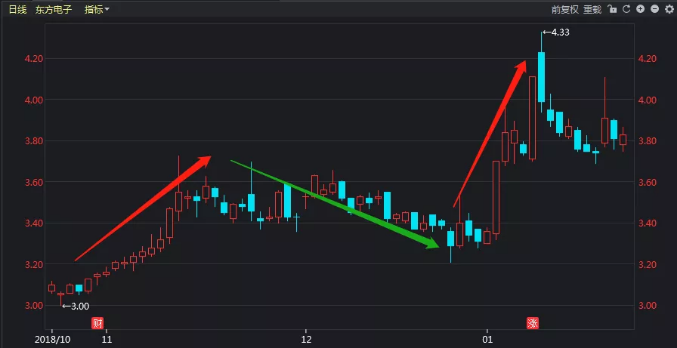
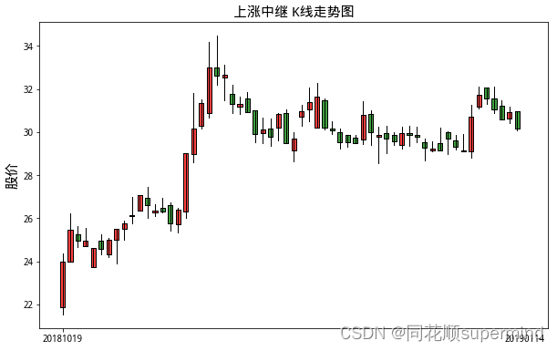
“W底”,“多头上涨”,“趋势回踩”,”上涨中继“这些都是常见的K线形态,以”上涨中继“为例,当股价快速上涨后,出现盘整形态而非顶部形态,预示股价还会进一步上涨,那么本节主要讲述”上涨中继”形态是否能够预测未来股价上涨,以及如何应用“上涨中继”形态,来快速选股。
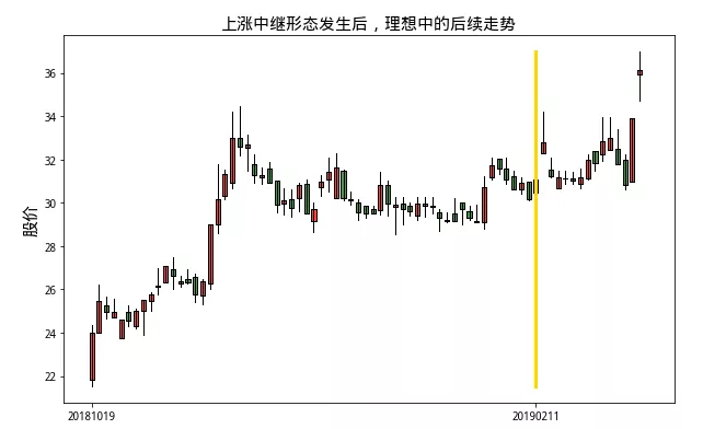
第一步:选取一段标准的“上涨中继”形态K线图

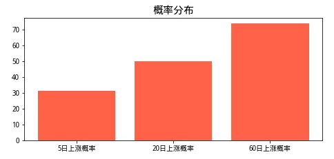
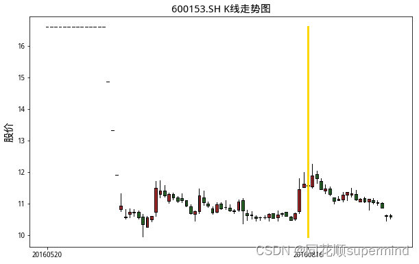
第二步:形态验证,在历史行情中寻找相似度高达0.8的K线图,并计算后5日、20日、60日的收益率。分析: 1.历史4年中“上涨中继”形态发生后,后5日上涨概率仅为30%,后20上涨概率也仅为50%,但后60日上涨概率高达70% 2.形态发生后,5日收益率均值为-2.45%,20日收益率均值仅为0.97%,但后60日收益率均值高达15.60% 并初步得出结论: 上涨中继形态发生后,技术分析者应该尽量选择低位介入,并且持有一段时间,而不是早早离场。


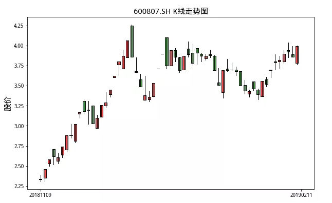
第三步:形态选股应用,我们认为“上涨中继”是一个较优质的中线买入机会,我们对全市场个股进行“上涨中继”形态选股,寻找出相似度最高的股票:ST天业,相似度为0.895,K线形态符合“上涨中继”,如下:
结束语:
"相似K线"技术相比于传统的K线组合而言更具技术性,其还有较多的运用空间,比如:运用顶部形态来监控个股潜在的下跌风险,运用相似度来监控个股是否脱离大盘走势,研究各类形态的上涨预测能力,并应用于选股等等。 注意:文中对股价的预测来源于模型运算结果,不构成投资建议!
参考文献:
-日本蜡烛图技术 [美] 史蒂夫·尼森
点击获取内容完整源码(仅支持PC):
点击→机器学习
微信扫码,在线阅读~:

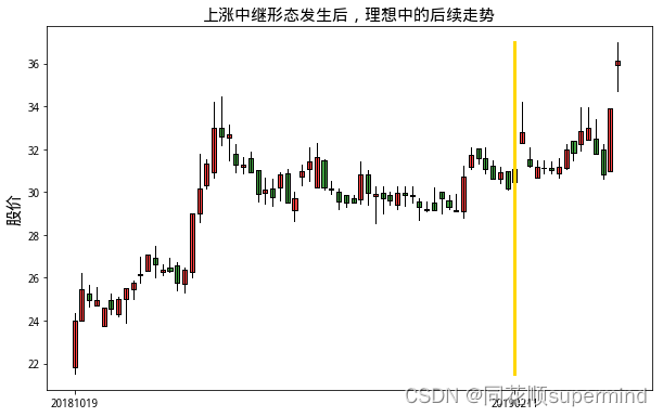
形态验证:快速上涨后,出现盘整形态,后续上涨的可能性多大?
data = get_price('603383.SH',None,'20190114','1d',['open','high','low','close'],bar_count=60,is_panel =1)

startdate ='20181019'
enddate ='20190114'

import numpy as np
import matplotlib.pyplot as plt
from matplotlib.finance import candlestick2_ohlc
import datetime

close1 = data['close']
open1 = data['open']
high1 = data['high']
low1 = data['low']

#画图
fig,ax = plt.subplots(figsize = (10,6.18),facecolor='white')
fig.subplots_adjust()

ticks = ax.set_xticks([0,60])
labels = ax.set_xticklabels([startdate,enddate], fontsize=10)


plt.yticks()
plt.title("{} K线走势图".format('上涨中继'),fontsize = 15)
plt.ylabel("股价",fontsize = 15)
candlestick2_ohlc(ax,open1,high1,low1,close1,width=0.6,colorup='red',colordown='green')
(<matplotlib.collections.LineCollection at 0x7f8b266317f0>, <matplotlib.collections.PolyCollection at 0x7f8b26983da0>)
data = get_price('603383.SH','20181019','20190211','1d',['open','high','low','close'],is_panel =1)

startdate ='20181019'
enddate ='20190211'

import numpy as np
import matplotlib.pyplot as plt
from matplotlib.finance import candlestick2_ohlc
import datetime

close1 = data['close']
open1 = data['open']
high1 = data['high']
low1 = data['low']

#画图
fig,ax = plt.subplots(figsize = (10,6.18),facecolor='white')
fig.subplots_adjust()

ticks = ax.set_xticks([0,60])
labels = ax.set_xticklabels([startdate,enddate], fontsize=10)

#支撑线
plt.plot([60,60],[np.min(low1),np.max(high1)],'gold',linewidth=3)

plt.yticks()
plt.title("{}形态发生后,理想中的后续走势".format('上涨中继'),fontsize = 15)
plt.ylabel("股价",fontsize = 15)
candlestick2_ohlc(ax,open1,high1,low1,close1,width=0.6,colorup='red',colordown='green')
(<matplotlib.collections.LineCollection at 0x7f8b25d5b978>, <matplotlib.collections.PolyCollection at 0x7f8b25d5b780>)
data = get_price('603383.SH',None,'20190114','1d',['open','high','low','close'],bar_count=60,is_panel =1)

close1 = data['close']
open1 = data['open']
high1 = data['high']
low1 = data['low']


indexcode = '000300.SH'
startdate = '20140101'
enddate = '20190201'
stocklist = get_index_stocks(indexcode,enddate)
data = get_price(stocklist,startdate,enddate,'1d',['open','high','low','close'],is_panel =1)
#收盘价
closedf = data['close'].fillna(0)
opendf = data['open'].fillna(0)
highdf = data['high'].fillna(0)
lowdf = data['low'].fillna(0)


dt = pd.DataFrame(columns=['stock','startdate','enddate','T'])

trade = list(closedf.index.strftime('%Y%m%d'))
num = trade.index(enddate)
stocklist = list(closedf.columns)
y=0
import datetime
for d in list(range(60,num-20,20)):
    print(d,num)
    close2 = closedf.iloc[d-59:d+1]
    opens2 = opendf.iloc[d-59:d+1]
    high2 = highdf.iloc[d-59:d+1]
    low2 = lowdf.iloc[d-59:d+1]

    for s in stocklist:
        corropen = round(np.corrcoef(open1,opens2[s])[0][1],3)
        corrhigh = round(np.corrcoef(high1,high2[s])[0][1],3)
        corrlow = round(np.corrcoef(low1,low2[s])[0][1],3)
        corrclose = round(np.corrcoef(close1,close2[s])[0][1],3)

        #综合值
        T = (corropen+corrhigh+corrlow+corrclose)/4
        startdate = trade[d-59]
        enddate = trade[d+1]
        dt.loc[y] = [s,startdate,enddate,T]
        y+=1

dt = dt.fillna(0)
dt = dt.sort_values(by='T',ascending=False)
dt
60 1242 80 1242 100 1242 120 1242 140 1242 160 1242 180 1242 200 1242 220 1242 240 1242 260 1242 280 1242 300 1242 320 1242 340 1242 360 1242 380 1242 400 1242 420 1242 440 1242 460 1242 480 1242 500 1242 520 1242 540 1242 560 1242 580 1242 600 1242 620 1242 640 1242 660 1242 680 1242 700 1242 720 1242 740 1242 760 1242 780 1242 800 1242 820 1242 840 1242 860 1242 880 1242 900 1242 920 1242 940 1242 960 1242 980 1242 1000 1242 1020 1242 1040 1242 1060 1242 1080 1242 1100 1242 1120 1242 1140 1242 1160 1242 1180 1242 1200 1242 1220 1242
Out[29]:
| stock | startdate | enddate | T | |
|---|---|---|---|---|
| 2046 | 601328.SH | 20140703 | 20140926 | 0.92825 |
| 2066 | 601788.SH | 20140703 | 20140926 | 0.92750 |
| 14425 | 000703.SZ | 20171208 | 20180312 | 0.92525 |
| 13279 | 002460.SZ | 20170811 | 20171110 | 0.92400 |
| 1859 | 002142.SZ | 20140703 | 20140926 | 0.92225 |
| 3194 | 600637.SH | 20141031 | 20150127 | 0.91750 |
| 1916 | 600000.SH | 20140703 | 20140926 | 0.91350 |
| 9898 | 603986.SH | 20160816 | 20161117 | 0.91200 |
| 4871 | 002310.SZ | 20150429 | 20150724 | 0.91000 |
| 4977 | 600482.SH | 20150429 | 20150724 | 0.90850 |
| 9533 | 601166.SH | 20160719 | 20161020 | 0.90450 |
| 11941 | 601228.SH | 20170317 | 20170616 | 0.90325 |
| 14971 | 601838.SH | 20180108 | 20180411 | 0.90300 |
| 5383 | 601985.SH | 20150528 | 20150821 | 0.90200 |
| 1921 | 600015.SH | 20140703 | 20140926 | 0.90075 |
| 6901 | 000002.SZ | 20151124 | 20160224 | 0.90000 |
| 12625 | 000703.SZ | 20170616 | 20170908 | 0.89900 |
| 14093 | 603260.SH | 20171013 | 20180108 | 0.89825 |
| 5310 | 600886.SH | 20150528 | 20150821 | 0.89750 |
| 3776 | 600438.SH | 20141226 | 20150331 | 0.89675 |
| 1803 | 000069.SZ | 20140703 | 20140926 | 0.89625 |
| 2079 | 601901.SH | 20140703 | 20140926 | 0.89575 |
| 2022 | 601009.SH | 20140703 | 20140926 | 0.89500 |
| 11382 | 601939.SH | 20170113 | 20170418 | 0.89475 |
| 2082 | 601939.SH | 20140703 | 20140926 | 0.89475 |
| 2089 | 601998.SH | 20140703 | 20140926 | 0.89350 |
| 2453 | 002044.SZ | 20140828 | 20141128 | 0.89300 |
| 1932 | 600036.SH | 20140703 | 20140926 | 0.89125 |
| 240 | 601225.SH | 20140103 | 20140404 | 0.89075 |
| 9416 | 600000.SH | 20160719 | 20161020 | 0.88725 |
| ... | ... | ... | ... | ... |
| 10657 | 600233.SH | 20161117 | 20170217 | -0.86350 |
| 16076 | 600438.SH | 20180511 | 20180806 | -0.86425 |
| 5164 | 002230.SZ | 20150528 | 20150821 | -0.86425 |
| 2738 | 000895.SZ | 20140926 | 20141226 | -0.86475 |
| 7396 | 600674.SH | 20151222 | 20160323 | -0.86825 |
| 11925 | 601021.SH | 20170317 | 20170616 | -0.86825 |
| 14339 | 601216.SH | 20171110 | 20180205 | -0.86850 |
| 10763 | 601688.SH | 20161117 | 20170217 | -0.86875 |
| 11936 | 601198.SH | 20170317 | 20170616 | -0.86900 |
| 14379 | 601901.SH | 20171110 | 20180205 | -0.86900 |
| 14863 | 600339.SH | 20180108 | 20180411 | -0.87000 |
| 9747 | 600153.SH | 20160816 | 20161117 | -0.87000 |
| 365 | 002236.SZ | 20140207 | 20140507 | -0.87075 |
| 15448 | 600157.SH | 20180312 | 20180608 | -0.87100 |
| 12086 | 002558.SZ | 20170418 | 20170714 | -0.87575 |
| 12015 | 000503.SZ | 20170418 | 20170714 | -0.87675 |
| 15385 | 002555.SZ | 20180312 | 20180608 | -0.87825 |
| 10725 | 601021.SH | 20161117 | 20170217 | -0.87975 |
| 14711 | 000413.SZ | 20180108 | 20180411 | -0.88000 |
| 16123 | 601012.SH | 20180511 | 20180806 | -0.88050 |
| 16553 | 002044.SZ | 20180709 | 20181009 | -0.88150 |
| 16244 | 000983.SZ | 20180608 | 20180903 | -0.88225 |
| 15977 | 002450.SZ | 20180511 | 20180806 | -0.88375 |
| 16209 | 000402.SZ | 20180608 | 20180903 | -0.88650 |
| 15993 | 002673.SZ | 20180511 | 20180806 | -0.89125 |
| 3392 | 002625.SZ | 20141128 | 20150303 | -0.89250 |
| 209 | 600867.SH | 20140103 | 20140404 | -0.90050 |
| 10890 | 002602.SZ | 20161215 | 20170317 | -0.90350 |
| 12097 | 002797.SZ | 20170418 | 20170714 | -0.91150 |
| 8847 | 600153.SH | 20160520 | 20160816 | -0.91225 |
17700 rows × 4 columns
In [30]:
for s in [0,-1]:
    stock = dt.iloc[s].stock
    startdate = dt.iloc[s].startdate
    enddate = dt.iloc[s].enddate

    import numpy as np
    import matplotlib.pyplot as plt
    from matplotlib.finance import candlestick2_ohlc
    import datetime
    s = stock

    trade = list(closedf.index.strftime('%Y%m%d'))
    num = trade.index(enddate)
    close1 = closedf[s].iloc[num-59:num+21]
    open1 = opendf[s].iloc[num-59:num+21]
    high1 = highdf[s].iloc[num-59:num+21]
    low1 = lowdf[s].iloc[num-59:num+21]

    #画图
    fig,ax = plt.subplots(figsize = (10,6.18),facecolor='white')
    fig.subplots_adjust()
    #支撑线
    plt.plot([60,60],[np.min(low1),np.max(high1)],'gold',linewidth=3)
    ticks = ax.set_xticks([0,60])
    labels = ax.set_xticklabels([startdate,enddate], fontsize=10)

    plt.yticks()
    plt.title("{} K线走势图".format(s),fontsize = 15)
    plt.ylabel("股价",fontsize = 15)
    candlestick2_ohlc(ax,open1,high1,low1,close1,width=0.6,colorup='red',colordown='green')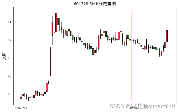
highdt = dt[dt['T']>0.8]
highdt['code'] = highdt.index
highdt['buyprice'] = highdt['code'].apply(lambda x:closedf[list(highdt['stock'])[list(highdt['code']).index(x)]].iloc[list(highdt['code']).index(x)])
highdt = highdt[highdt['buyprice']!=0]
highdt['5day'] = highdt['code'].apply(lambda x:closedf[list(highdt['stock'])[list(highdt['code']).index(x)]].iloc[list(highdt['code']).index(x)+5])
highdt['20day'] = highdt['code'].apply(lambda x:closedf[list(highdt['stock'])[list(highdt['code']).index(x)]].iloc[list(highdt['code']).index(x)&#
最低0.47元/天 解锁文章


 807
807


 被折叠的 条评论
为什么被折叠?
被折叠的 条评论
为什么被折叠?
 到【灌水乐园】发言


