线性模型之线性分类器之间的博弈

接着上一篇博客，继续聊聊线性分类器。虽然线性分类器是机器学习的入门级算法，但是最近重新看有关机器学习的书籍的时候，发现就算是入门级的算法，里面的门道依旧很多，写这篇博客时，也只是觉得自己了解一些皮毛。没办法，毕竟一口吃不了一个大胖子，知识是慢慢积累的。大佬都是养成的！！！哈哈

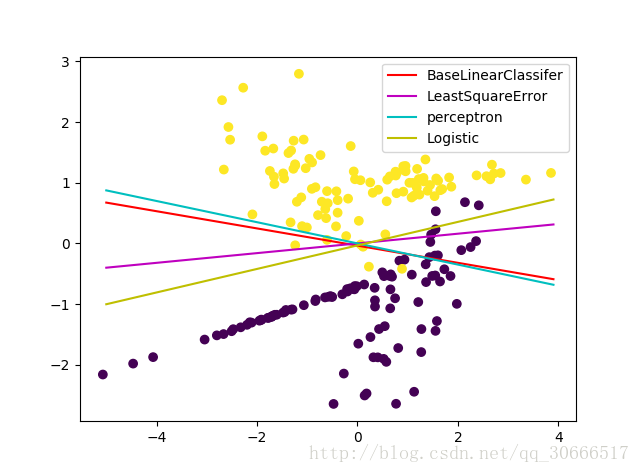
这篇博客主要比较4种线性分类器的不同。分别是上篇博客介绍的基本线性分类器，最小二乘分类器，感知器，以及Logistic线性分类器。基本线性分类器就如同上篇博客介绍那样，从几何角度去得到超平面的法向量以及阈值t。最小二乘分类器不再是从几何角度求解权重向量y=X*w,X是输入的训练集特征，w是待求解向量。按照线性代数的知识可以得到w=inver(X)*w,但是X不一定可逆，但是从矩阵论角度X存在广义逆矩阵。最小二乘法本质上还是是平方误差之和最小化的近似解，（矛盾方程组无解，实际中都是这样，只能求近似解），那么最终得到的解析解是:w=inv(X.T*X)*X.T.*y。感知器分类器属于迭代算法了，在训练数据集上进行迭代。对于每个错分类的实例，都对权重向量进行调整。假设xi是一正例，label=1，若错分类为负例，即w.x<0,那么需要增加权重向量使得w.x>0,使之能正确的分类。权重更新法则为w=w+a*xi(a是学习率)，这样在整个训练集上进行迭代，直到所有的训练样例都被正确分类。（实际上如果数据不是严格线性可分的，感知器是不可能收敛的，当然也存在过拟合的问题）。最后Logsitic线性分类器使用的是sklearn库封装好的算法，求解权重向量时，采用的是梯度下降算法（计算机迭代求解的数值解）。

若表示之前都很少用python面向对象的思想编程，这次尝试使用面向对象的思想。中间bug很多，从构思到完全实现花了将近4个小时。雪崩！！！下面贴图给出，四种不同的线性分类器在同一个二类数据集上得到的决策边界。构造的数据集是2维特征，因为方便可视化，你懂的。

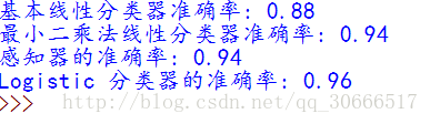
看一下性能

# !/usr/bin/env python
# -*- coding:utf-8 -*- 
# Author: wsw
# 线性分类器学习
from sklearn.model_selection import train_test_split
from sklearn.linear_model import LogisticRegression
from sklearn.datasets import make_classification
from sklearn.metrics import accuracy_score
import numpy as np
import numpy.linalg as lin
import matplotlib.pyplot as plt


# 定义一个基本线性分类器
class BaseLinearClassifier:
	def __init__(self, w=np.zeros((2, 1))):
		# 私有属性不允许多继承!!!
		self.weight = w

	# 查看权重系数
	@property
	def get_weight(self):
		return self.weight

	# 训练函数
	def fit(self, xtrain, ytrain):
		# 得到正例索引
		index1 = np.where(ytrain == 1)
		# 正例中心
		pos_centriod = np.mean(xtrain[index1[0]], axis=0)
		# 得到反例索引
		index2 = np.where(ytrain == 0)
		# 反例中心
		neg_centriod = np.mean(xtrain[index2[0]], axis=0)
		# 得到权重向量
		self.weight = pos_centriod - neg_centriod
		# 计算阈值t
		T = np.dot(self.weight, 1 / 2 * (pos_centriod + neg_centriod))
		return T

	# 准确率测试
	def score(self, xtest, ytest, threshold):
		# 测试集预测类别
		predict = []
		for i in xtest:
			if np.dot(i, self.weight) >= threshold:
				predict.append(1)
			else:
				predict.append(0)
		accuracy = accuracy_score(ytest, predict)
		return accuracy


# 定义最小二乘线性分类器
class LeastSquareError(BaseLinearClassifier):
	def __init__(self):
		super().__init__()

	# 重写训练方法
	# 利用正规方程得到解析解
	def fit(self, xtrain, ytrain):
		self.weight = np.dot(np.matmul(lin.inv(np.matmul(xtrain.T, xtrain)), xtrain.T), ytrain)

	# 准确率测试
	def score(self, xtest, ytest, threshold=0):
		predict = []
		for i in xtest:
			if np.dot(i, self.weight) > 0:
				predict.append(1)
			else:
				predict.append(0)
		accuracy = accuracy_score(ytest, predict)
		return accuracy

	@property
	def get_weight(self):
		return self.weight


# 感知器分类器
class Percptron(BaseLinearClassifier):
	def __init__(self, learning_rate=0.1):
		super().__init__(np.random.rand(2, 1))
		self.__learning_rate = learning_rate

	def fit(self, xtrain, ytrain):
		# 找到训练集中的所有正例
		indexs = np.where(ytrain == 1)
		pos = xtrain[indexs[0], :]
		# 对于误分类的正例进行权重学习
		# 直到所有正例都被正确分类，退出迭代， 否则达到最大迭代次数，退出迭代
		count = 0
		for ite in range(500):
			for i in pos:
				if np.dot(i, self.weight) < 0:
					self.weight += self.__learning_rate*np.array(i).reshape(-1, 1)
				else:
					# 正确分类个数加1
					count += 1
			if count == len(indexs[0]):
				break

	def score(self, xtest, ytest, threshold=0):
		predict = []
		for i in xtest:
			if np.dot(i, self.weight) >= 0:
				predict.append(1)
			else:
				predict.append(0)
		accuracy = accuracy_score(ytest, predict)
		return accuracy

	@property
	def get_weight(self):
		return self.weight


def main():
	# 构造数据
	rowdata, label = make_classification(200, 2, n_redundant=0, random_state=31)
	plt.scatter(rowdata[:, 0], rowdata[:, 1], c=label)
	# split data
	xtrain, xtest, ytrain, ytest = train_test_split(rowdata, label, test_size=0.25, random_state=33)
	# 构造一个基本线性分类器
	baseLR = BaseLinearClassifier()
	# 训练,返回阈值T
	T = baseLR.fit(xtrain, ytrain)
	# 准确率评价
	accuracy_baseLR = baseLR.score(xtest, ytest, T)
	print('基本线性分类器准确率:', accuracy_baseLR)
	# 画出基本线性分类器决策边界
	w = baseLR.get_weight
	x = np.arange(-5, 4, 0.1)
	y = (T - x * w[0]) / w[1]
	plt.plot(x, y, c='r', label='BaseLinearClassifer')

	# 构造最小二乘线性分类器
	lsqLR = LeastSquareError()
	lsqLR.fit(xtrain, ytrain)
	accuracy_lsqLR = lsqLR.score(xtest, ytest)
	print('最小二乘法线性分类器准确率:', accuracy_lsqLR)
	# 得到权重系数
	w1 = lsqLR.get_weight
	x1 = np.arange(-5, 4, 0.1)
	y1 = -x1 * w1[0] / w1[1]
	plt.plot(x1, y1, c='m', label='LeastSquareError')

	# 构造感知器分类器
	perctron = Percptron()
	perctron.fit(xtrain, ytrain)
	accuracy_percptron = perctron.score(xtest, ytest)
	print('感知器的准确率:', accuracy_percptron)
	w2 = perctron.get_weight
	x2 = np.arange(-5, 4, 0.1)
	y2 = -x1 * w2[0] / w2[1]
	plt.plot(x2, y2, c='c', label='perceptron')

	# 构造logistic Classifier
	lr = LogisticRegression()
	lr.fit(xtrain, ytrain)
	print('Logistic 分类器的准确率:', lr.score(xtest, ytest))
	w3 = lr.coef_
	b = lr.intercept_
	x3 = np.arange(-5, 4, 0.1)
	y3 = -(x3*w3[0, 0] + b)/w3[0, 1]
	plt.plot(x3, y3, c='y', label='Logistic')
	plt.legend()
	plt.show()
	pass


if __name__ == '__main__':
	main()
	pass