Local density adaptive similarity measurement for spectral clustering

代码：matlab Local-density-adaptive-similarity-measurement-for-spectral-clustering

摘要

相似度度量对谱聚类的性能至关重要。通常采用高斯核函数作为相似度度量。然而，在核参数固定的情况下，两个数据点之间的相似性仅由它们的欧氏距离决定，并不适应它们周围的环境。本文提出了一种局部密度自适应相似度度量方法，该方法利用两个数据点之间的局部密度来扩展高斯核函数。所提出的相似度度量满足聚类假设，并具有放大聚类内相似度的效果，从而使亲和矩阵（邻接矩阵）清晰地成为块对角线。在合成数据集和真实数据集上的实验结果表明，采用局部密度自适应相似度度量的谱聚类算法优于传统的谱聚类算法、基于路径的谱聚类算法和自调优谱聚类算法。

2. Overview of spectral clustering

Given a set of $n$ data points X = { x 1 , x 2 , … , x n } X=\left\{x_{1}, x_{2}, \ldots, x_{n}\right\} X={x1​,x2​,…,xn​}, the objective of clustering is to divide data points into different clusters, where data points in the same cluster are similar to each other. According to a specific similarity measure, we have the affinity matrix $S\in {\mathfrak{R}}^{n\times n}$. From $S$, we can construct an undirected graph $G=(V,E)$ with each vertex $v_i\in V$ corresponding to the data point $x_i$ and each edge $e(i,j)\in E$ carries a weight $S_{ij}$ which represents the similarity between point $x_i$ and $x_j$. The clustering problem is equivalent to choosing a partition $C_1,C_2,\dots ,C_k$ of $G$ which minimizes a specific objective function such as RatioCut (Hagen and Kahng, 1992), MinmaxCut (Ding et al., 2001), and the Ncut (Shi and Malik, 2000 ). The performances of these three objective functions are input dependent: if clusters are well separated, all the three give very similar and accurate results; when clusters are marginally separated, NCut and MinMaxCut give better results; when clusters overlap significantly, MinMaxCut tend to give more compact and balanced clusters (Ding, 2004). In this paper, we use the mostly often adopted Ncut. It was shown in (Wagner and Wagner, 1993) that the minimization of Ncut is NP-hard. According to Rayleigh-Ritz theory (Lütkepohl, 1997), it is possible to find an approximate solution. In solving this, we need to define the normalized Laplacian matrix $L=D^{-\frac{1}{2}}S{D}^{-\frac{1}{2}}$ where $D$ is a diagonal matrix with $D_{ii}=$ ${\sum }_{j=1}^n{S}_{ij}$. Then, the approximate solution could be derived from the leading eigenvectors of $L$. The use of Laplacian matrix eigenvector for approximating the graph minimum cut is called spectral clustering. A complete overview of spectral clustering can be found in (Luxburg, 2007).

给定一组$n$个数据点 X = { x 1 , x 2 , … , x n } X=\left\{x_{1}, x_{2}, \ldots, x_{n}\right\} X={x1​,x2​,…,xn​}，聚类的目的是将数据点划分为不同的集群，其中同一集群中的数据点彼此相似。根据特定的相似性度量，我们有亲和矩阵 $S\in {\mathfrak{R}}^{n\times n}$。从$S$，我们可以构造一个无向图$G=(V,E)$，每个顶点$v_i\in V$对应数据点$x_i$和每条边$e(i,j)\in E$ 带有一个权重 $S_{ij}$，它表示点 $x_i$ 和 $x_j$ 之间的相似度。聚类问题等价于选择 $G$ 的分区 $C_1,C_2,\dots ,C_k$ 最小化特定目标函数，例如 RatioCut (Hagen and Kahng, 1992), MinmaxCut （Ding 等人，2001 年）和 Ncut（Shi 和 Malik，2000 年）。这三个目标函数的性能取决于输入：如果集群分离得很好，那么这三个目标函数都会给出非常相似和准确的结果；当簇被边缘分离时，NCut 和 MinMaxCut 给出更好的结果；当集群显着重叠时，MinMaxCut 倾向于给出更紧凑和平衡的集群（Ding，2004）。在本文中，我们使用最常用的 Ncut。 (Wagner and Wagner, 1993) 表明 Ncut 的最小化是 NP 难的。根据 Rayleigh-Ritz 理论 (Lütkepohl, 1997)，可以找到一个近似解。在解决这个问题时，我们需要定义归一化拉普拉斯矩阵$L=D^{-\frac{1}{2}}S{D}^{-\frac{1}{2}}$ 其中 $D$ 是对角矩阵$D_{ii}=$${\sum }_{j=1}^n{S}_{ij}$。然后，可以从 $L$ 的前导特征向量导出近似解。使用拉普拉斯矩阵特征向量来逼近图的最小割称为谱聚类。谱聚类的完整概述可在 (Luxburg, 2007) 中找到。

The most commonly used similarity measure, the Gaussian kernel function, is defined as $S_G\left(x_i,x_j\right)=\exp \left(-d{\left(x_i,x_j\right)}^2/2{\sigma }^2\right)$, where $d\left(x_i,x_j\right)$ is the Euclidean distance between data points $x_i$ and $x_j$, and $\sigma$ is the kernel parameter (Shi and Malik, 2000). The obvious drawback of $S_G$ is that the scaling parameter $\sigma$ is fixed, thus the similarity between two points is only determined by their Euclidean distance, and does not vary with the change of the surroundings. An/ example is given in Fig. 1 (Fig. 2 in (Zelnik-Manor et al., 2004)). In Fig. 1(a), supposing $d(a,b)=d(a,c)$, then with the Gaussian kernel function we have $S_G(a,b)=S_G(a,c)$. Thus the clustering algorithm tends to cluster $a,b,c$ together. However, the fact is that $a,c$ are in the background cluster which is relatively sparse, while $b$ is in the tight cluster in the center.

最常用的相似性度量，高斯核函数，定义为 $S_G\left(x_i,x_j\right)=\exp \left(-d{\left(x_i,x_j\right)}^2/2{\sigma }^2\right)$， 其中 $d\left(x_i,x_j\right)$ 是数据之间的欧式距离点 $x_i$ 和 $x_j$，$\sigma$ 是内核参数 (Shi and Malik, 2000)。 $S_G$ 的明显缺点是缩放参数 $\sigma$ 是固定的，因此两点之间的相似度仅由它们的欧几里德距离决定，不随周围环境的变化而变化。图 1 给出了一个示例（Zelnik-Manor 等人，2004 年的图 2）。在图 1(a) 中，假设 $d(a,b)=d(a,c)$，那么使用高斯核函数我们有 $S_G(a,b)=S_G(a,c)$。因此，聚类算法倾向于将$a、b、c$ 聚类在一起。然而，事实是$a、c$在背景簇中，相对稀疏，而$b$在中心的紧密簇中。

Zelnik-Manor et al. proposed a local scale similarity measure $S_T\left(x_i,x_j\right)=\exp \left(-d{\left(x_i,x_j\right)}^2/{\sigma }_i{\sigma }_j\right)$, where ${\sigma }_i$ is the distance between point $x_i$ and its $k$ th nearest neighbor (Zelnik-Manor et al., 2004). With $S_T$, in Fig. 1, we have ${\sigma }_c>{\sigma }_b$, so ${\sigma }_a{\sigma }_c>{\sigma }_a{\sigma }_b$, point $a$ gets closer to point $c$ than to point $b$. This is just the information required for separation. The effect of local scaling can be seen from the comparison of Fig. 1(b) with Fig. 1（c）.

Zelnik-Manor 等人提出了一种局部尺度相似性度量 $S_T\left(x_i,x_j\right)=\exp \left(-d{\left(x_i,x_j\right)}^2/{\sigma }_i{\sigma }_j\right)$， 其中 ${\sigma }_i$ 是点 $x_i$ 与其第 $k$ 个最近邻点之间的距离（Zelnik-Manor等人，2004）。对于 $S_T$，在图 1 中，我们有 ${\sigma }_c>{\sigma }_b$，所以 ${\sigma }_a{\sigma }_c>{\sigma }_a{\sigma }_b$, 点 $a$ 比点 $b$ 更接近点 $c$。这只是分离所需的信息。从图1(b)与图1（c）的比较可以看出局部缩放的效果。

The corresponding spectral clustering based on this local scale similarity measure is called self-tuning spectral clustering (SCST) (Zelnik-Manor et al., 2004). Since the adaptive local scale parameter reflects the local information properly, SC-ST works well on the data with multiple scales, e.g., Fig. 1（c）. It reveals that the surroundings of two data points have high impact on their similarity.

基于这种局部尺度相似性度量的相应谱聚类称为自调整谱聚类 (SCST) (Zelnik-Manor et al., 2004)。由于自适应局部尺度参数正确反映了局部信息，因此 SC-ST 在具有多个尺度的数据上效果很好，例如，图 1（c）。它揭示了两个数据点的周围环境对它们的相似性有很大的影响。

However, the local scale parameter in SC-ST, the distance to a nearby neighbor, is still a Euclidean distance factor and does not help in many cases. For example, on the toy data set in Fig. 2, consider three data points $a,b,c$ with $d(a,b)=d(a,c)$ in the Euclidean space (see Fig. 3). Following the clustering assumption, the similarity between $a$ and $b$ should be higher than the similarity between $a$ and $c$, since point $a$ is in the same cluster with point $b$ rather than point c. Unfortunately, SC-ST does not work, since the local statistics surrounding point $b$ and $c$ are similar, leading to $S_T(a,b)=-S_T(a,c)$. It can not make any contribution to clustering better than using $S_G$, thus SC-ST fails to produce the correct clustering result (see Fig. 3).

然而，SC-ST 中的局部尺度参数，即到附近邻居的距离，仍然是欧几里得距离因子，在许多情况下没有帮助。例如，在图 2 的玩具数据集上，考虑欧几里得空间中的三个数据点 $a,b,c$，$d(a,b)=d(a,c)$（见图 3） .根据聚类假设，$a$ 和 $b$ 之间的相似度应该高于 $a$ 和 $c$ 之间的相似度，因为点 $a$ 与点 $b$ 而不是点 c 在同一个聚类中。不幸的是，SC-ST 不起作用，因为围绕点 $b$ 和 $c$ 的局部统计数据相似，导致 $S_T(a,b)=-S_T(a,c)$。它不能比使用 $S_G$ 更好地对聚类做出任何贡献，因此 SC-ST 无法产生正确的聚类结果（见图 3）。

The path-based similarity used in path based clustering (Fischer and Buhmann, 2003) is defined as followS: $S_P\left(x_i,x_j\right)={\max }_{p\in {\rho }_{ij}}$ $\left\{{\min }_{1⩽h<|p|}d\left(x_{p[h]},x_{p[h+1]}\right)\right\}$ where ${\wp }_{ij}$ denotes the set of all paths from $x_i$ to $x_j,p[h]$ denotes the $h$ th point along the path $p$ from $x_i$ to $x_j$. This $x_i$ to $x_j,p[h]$ denotes the $h$ th point along the path $p$ from $x_i$ to $x_j$. This tance between two points, they should be considered as in one cluster if they are connected by a set of successive points in dense regions. This is intuitively reasonable. However, it is not robust enough against noise and outliers (Chang and Yeung, 2008).

基于路径的聚类（Fischer and Buhmann, 2003）中使用的基于路径的相似性定义如下： $S_P\left(x_i,x_j\right)={\max }_{p\in {\rho }_{ij}}$ $\left\{{\min }_{1⩽h<|p|}d\left(x_{p[h]},x_{p[h+1]}\right)\right\}$ 其中 ${\wp }_{ij}$ 表示从 $x_i$ 到 $x_j$ 的所有路径的集合，$p[h]$ 表示沿路径 $p$ 的第 $h$ 个点从 $x_i$ 到 $x_j$。这 $x_i$ 到 $x_j，p[h]$ 表示从 $x_i$ 到 $x_j$ 的路径 $p$ 上的第 $h$ 个点。两点之间的这种距离，如果它们由密集区域中的一组连续点连接，则应将它们视为一个簇。这在直觉上是合理的。然而，它对噪声和异常值的鲁棒性不够（Chang 和 Yeung，2008 年）。

4. Local density adaptive similarity measure

一个好的相似性度量应该是自适应于相关点的邻域。我们所提出的方法是基于以下观察:如果两个点分布在同一簇中，它们是在同一密度相对较高的区域内。也就是说，两个点落在同一簇中，因为它们之间有许多点将它们“粘合”在一起。为了反映两个数据点之间的“粘合”效应，我们定义了共同近邻(Common-Near-Neighbor, CNN)措施。

Definition 1. $CNN(a,b)$ is the number of the points in the join region of the $\epsilon$-neighborhoods around points $a$ and $b$, where the $\epsilon$ neighborhood of one point represents the sphere region around that point of specified radius $\epsilon$.

$CNN(a,b)$ 是点 $a$ 和 $b$ 周围 $\epsilon$ 邻域的连接区域中的点数，其中一个点的 $\epsilon$ 邻域表示围绕指定半径 $\epsilon$ 的那个点的球体区域。

$CNN(a,b)$ shows the local density between points $a$ and $b$, which can be used to distinguish points within the same cluster from points among different clusters. For example, as shown in Fig. 4, points $a$ and $b$ have more shared neighbors than points $a$ and $c$, so we will have $CNN(a,b)>CNN(a,c)$, which contains strong information for data partition.

$CNN(a,b)$ 显示了点 $a$ 和 $b$ 之间的局部密度，可以用来区分同一簇内的点和不同簇间的点。例如，如图 4 所示，点 $a$ 和 $b$ 的共享邻居比点 $a$ 和 $c$ 多，因此我们将有 $CNN(a,b)>CNN(a,c)$，其中包含数据分区的强信息。

The local density adaptive similarity measure between a pair of points is thus defined as:

因此，一对点之间的局部密度自适应相似性度量定义为：
$$S_L\left(x_i,x_j\right)=\{\begin{array}{ll}\exp \left(-\frac{d{\left(x_i,x_j\right)}^2}{2{\sigma }^2\left(CNN\left(x_i,x_j\right)+1\right)}\right)& i\ne j\\ 0& i=j\end{array}$$
The proposed similarity measure has the following properties:

建议的相似性度量具有以下特性：

(1) If $d\left(x_i,x_j\right)⩾2\epsilon$, then $S_L\left(x_i,x_j\right)=S_G\left(x_i,x_j\right)$, showing that the scale factor is a local one and does not affect far away data points.

(1) 如果 $d\left(x_i,x_j\right)⩾2\epsilon$，则 $S_L\left(x_i,x_j\right)=S_G\left(x_i,x_j\right)$，表明比例因子是局部的，不会影响远处的数据点。

(2) For two pairs of points $x_i,x_j$ and $x_m,x_n$, supposing $d\left(x_i,x_j\right)=$ $d\left(x_m,x_n\right)<2\epsilon$, but in fact $x_i,x_j$ are in the same dense region while $x_m,x_n$ are in different dense regions, then with very high probability we have $S_L\left(x_i,x_j\right)>S_L\left(x_m,x_n\right)$. For example, in Fig. $4,S_L(a,b)>S_L(a,c)$.

(2) 对于两对点 $x_i,x_j$ 和 $x_m,x_n$, 假设 $d\left(x_i,x_j\right)=$ $d\left(x_m,x_n\right)<2\epsilon$，但实际上$x_i,x_j$在同一个密集区域，而$x_m,x_n$ 位于不同的密集区域，那么很有可能我们有 $S_L\left(x_i,x_j\right)>S_L\left(x_m,x_n\right)$.例如，在图 $4中，S_L(a,b)>S_L(a,c)$。

Since clusters are dense regions of the data set, thus from (2) it can be seen that our defined similarity has an effect of amplifying the intra-cluster similarity. This is desirable for high quality clustering.

由于集群是数据集的密集区域，因此从（2）可以看出，我们定义的相似度具有放大集群内相似度的效果。这对于高质量的聚类是可取的。

Till now, to the best of our knowledge, there has been no quantitative metric on to what extent a similarity measure is good. However, it is believed that a good similarity function should make the affinity matrix as block diagonal as possible (and Poland, 2005). This is usually evaluated through visualizations of the affinity matrices. For the two-moon dataset, visualizations of the affinity matrices using the three different similarity functions are given in Fig. 5. Note that with our local density adaptive similarity measure, points in the same cluster obtain the highest similarities. It is the closest to the ideal block diagonal matrix (in which the value is 1 when two points are in the same cluster and 0 otherwise).

到目前为止，据我们所知，还没有关于相似性度量在多大程度上好的量化指标。然而，人们认为一个好的相似性函数应该使亲和矩阵(邻接矩阵)尽可能地成为块对角线。这通常通过亲和矩阵(邻接矩阵)的可视化来评估。对于双月数据集，图 5 给出了使用三种不同相似度函数的亲和度矩阵的可视化。请注意，使用我们的局部密度自适应相似度度量，同一簇中的点获得最高相似度。它最接近理想的块对角矩阵（其中两个点在同一个簇中时值为 1，否则为 0）。(亲和矩阵图像中元素越亮，对应数据点之间的相似度越高).(a)玩具数据集的散点图，(b) $S_G$计算的亲和矩阵，© $S_T$计算的亲和矩阵，(d) $S_L$计算的亲和矩阵。

The local density adaptive spectral clustering algorithm (SC-DA) is simply the ordinary spectral clustering algorithm using the new similarity measure $S_L$ in place $S_G$. This seemingly minor modification is in fact very significant as the clustering results can be improved effectively. The clustering result on the two moon dataset with our method is shown in Fig. 6. The groups now match the real solution well (Recall the result of SC-ST in Fig. 3. to see the superiority of our similarity for this dataset).

局部密度自适应谱聚类算法 (SC-DA) 只是使用新的相似性度量 $S_L$ 代替 $S_G$ 的普通谱聚类算法。这种看似微小的修改实际上非常重要，因为可以有效地改善聚类结果。使用我们的方法在两个月球数据集上的聚类结果如图 6 所示。这些组现在很好地匹配了真实的解决方案（回忆图 3 中 SC-ST 的结果。看看我们对这个数据集的相似性的优越性） .

5. Experiments

5.1. Parameter setting

在我们的实验中，$\sigma$的值是通过搜索欧氏距离总范围的10%到20%来设置的，并选择最紧密的聚类。k在SC-ST中从2到50不等，使用的是提供最紧密集群的k。通过线性回归的实证分析，SC-DA中的$\epsilon$ 设为:$\epsilon =20mea{n}_d+54mi{n}_d+13-ma{x}_n-6ma{x}_d-65mea{n}_n$， $ma{x}_d$，$mea{n}_d$和$mi{n}_d$是所有成对的数据点之间的最大距离，均值距离，最小距离，而$ma{x}_n$，$mea{n}_n$是每个数据点与其最近邻之间的是最大距离，均值距离。
使用NCUT，对称正则化拉普拉斯。

5.2. Experiments on synthetic data sets

将上述4个聚类方法（ SC, SC-ST, SC-PB and SC-DA）应用到3个2D和2个3D的合成数据集上。toy数据集

5.3. Experiments on real world data sets

将上述4个聚类方法（ SC, SC-ST, SC-PB and SC-DA）在UCI数据集和UPS数据集上测试。用Clustering Error(CE) 和Normalized Mutual Information(NMI)两个评估指标。

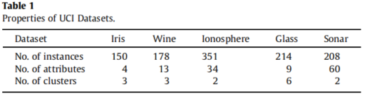
5.3.2. Results on UCI data sets

对来自UCI数据存储库(Asuncion and Newman, http://archive.ics.uci.edu/ml/)的四个真实数据集进行了实验。

5.3.3. Results on USPS data sets

对来自USPS数据库的手写数字进行了实验。将数字大小归一化，并以16px×16px灰度图像居中，数字空间的维数为256。它包含7291个训练实例和2007个测试实例。我们选择测试实例中的数字{0,8}、{3,5,8}、{1,2,3,4}和{0,2,4,6,7}作为子集，分别进行比较实验。