Tensorflow

一、Tensorflow优点和基础架构

1、优点

2、基础架构

二、Tensorflow核心概念

计算图、运算操作、变量、会话

1、计算图

1） 什么是计算图？

2） 计算图的构造流程

2、操作节点

3、变量

1） 变量的创建

2）变量的初始化

3）变量的保存和恢复

4、会话

三、Tensorflow 实现原理

四、Tensorflow扩展功能

1、自动求导

2、字图执行

3、计算图控制流

4、队列\容器

五、Tensorflow性能优化

1、运算操作节点重组和调度

2、异步计算支持（并行）

3、第三方计算库

4、三种并行计算模式

• 数据并行模式
  
• 模型并行模式
  
• 流水线并行模式
  
• 三种并行方式比较
  

六、深度学习框架

七、常用常量/变量/矩阵操作

import tensorflow as tf

"""打印hello world"""
a = tf.constant("hello world")
with tf.Session() as sees:
    print(sees.run(a))

# 基本常量操作
# 构造函数返回值就是常量节点的输出
a1 = tf.constant(2)
a2 = tf.constant(3)

# 启动默认计算图
with tf.Session() as sees:
    print('常量相加：', sees.run(a1 + a2))
    print('常量相乘：', sees.run(a1 * a2))

# 使用变量作为计算图输入
# 定义输入, tf.placeholder为占位符
a2 = tf.placeholder(tf.int16)
b2 = tf.placeholder(tf.int16)
# 定义操作
add = tf.add(a2, b2)
mul = tf.multiply(a2, b2)
# 启动会话
with tf.Session() as sees:
    print('变量相加：', sees.run(add, feed_dict={a2: 2, b2: 3}))
    print('变量相乘：', sees.run(mul, feed_dict={a2: 2, b2: 3}))

# 使用矩阵作为计算图输入
matrix1 = tf.constant([[2, 2]])
matrix2 = tf.constant([[1], [2]])

# 定义矩阵相乘操作
mul_mat = tf.matmul(matrix1, matrix2)

with tf.Session() as sees:
    print('矩阵相乘：', sees.run(mul_mat))
    

1、tf.placeholder()

八、Tensorflow构建KNN分类器

原理

Tensorflow实现KNN需要以下几步：

import numpy as np
import tensorflow as tf

# 这里使用TensorFlow自带的数据集作为测试，以下是导入数据集代码
from tensorflow.examples.tutorials.mnist import input_data

mnist = input_data.read_data_sets("/tmp/data/", one_hot=True)

Xtrain, Ytrain = mnist.train.next_batch(5000)  # 从数据集中选取5000个样本作为训练集
Xtest, Ytest = mnist.test.next_batch(200)  # 从数据集中选取200个样本作为测试集

# 输入占位符
xtr = tf.placeholder('float', [None, 784])
xte = tf.placeholder('float', [1, 784])

# 计算L1距离
distance = tf.reduce_sum(tf.abs(tf.add(xtr, tf.negative(xte))), axis=1)

# 获取最小距离的索引
pred_index = tf.arg_min(distance, 0)

# 分类精确度
acc = 0.

# 初始化变量
init = tf.global_variables_initializer()

# 启动会话
with tf.Session() as sees:
    sees.run(init)
    for i in range(Xtest.shape[0]):
        index = sees.run(pred_index, feed_dict={xtr: Xtrain, xte: Xtest[i, :].reshape(1, 784)})
        true = np.argmax(Ytest[i])  # 第i个样本的真实标签
        pred_x = np.argmax(Ytrain[index])  # 第i个样本的预测标签
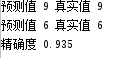
        print('预测值', pred_x, '真实值', true)
        if pred_x == true:
            acc += 1
    acc = acc / Xtest.shape[0]
    print('精确度', acc)

# 保存事件日志到tensorboard
writer = tf.summary.FileWriter("./logs", tf.get_default_graph())

writer.close()

九、Tensorboard可视化

1、WEB可视化

• E: 进入E盘
• cd E:\tensorflow_study\MNIST\logs 进入事件日志的上一级目录
• tensorboard.exe --logdir=E:\tensorflow_study\MNIST\logs
  
• 打开浏览器，输入localhost:6006
  

2、summary语句

十、Tensorflow实现一元线性回归

线性回归

import numpy as np
import pandas as pd
import tensorflow as tf
import matplotlib.pyplot as plt

"""读入数据"""

data=pd.read_csv(r'E:\tensorflow_study\MNIST\my_data\Advertising.csv')
#归一化数据
x=data['TV'],y=data['Sales']
x_mean=np.mean(x)
y_mean=np.mean(y)
x_std=np.std(x)
y_std=np.std(y)
x=(x-x_mean)/x_std
y=(y-y_mean)/y_std
x_train=x[1:150]
y_train=y[1:150]
x_test=x[150:200]
y_test=y[150:200]

# x_train = np.linspace(0,10,100) + np.random.uniform(-1.5,1.5,100)
# y_train = np.linspace(0,10,100) + np.random.uniform(-1.5,1.5,100)
# x_test = np.linspace(0,10,20) + np.random.uniform(-1.5,1.5,20)
# y_test = np.linspace(0,10,20) + np.random.uniform(-1.5,1.5,20)

"""数据可视化"""
plt.plot(x_train,y_train,'ro')
plt.plot(x_test,y_test,'b*')

"""构建计算图"""
with tf.Graph(). as_default():
    #1
    # 输入占位符
    with tf.name_scope('Input'):
        x=tf.placeholder('float',name='X')
        y=tf.placeholder('float',name='Y')

    # 2、前向计算和损失
    with tf.name_scope('Inference'):
        w=tf.Variable(tf.zeros([1]),name='weight')
        b = tf.Variable(tf.zeros([1]),name='bias')
        y_hat=tf.add(tf.multiply(w,x),b)
    with tf.name_scope('Loss'):
        loss_train= tf.reduce_mean(tf.pow(y_hat-y,2))/2

    #3训练，# 创建梯度下降优化器
    with tf.name_scope('Train'):
        optimizer=tf.train.GradientDescentOptimizer(learning_rate=0.01)
        #定义train节点，将优化器应用到loss_train
        trainOP=optimizer.minimize(loss_train)

    # 4、评估
    with tf.name_scope('Evaluate'):
        Evalloss=tf.reduce_mean(tf.pow(y_hat-y,2))/2


    # 添加初始化节点
    initOP=tf.global_variables_initializer()
    with tf.Session() as sees:
        sees.run(initOP)
        for i in range(1000):
            _,train_loss,train_w,train_b=sees.run([trainOP,loss_train,w,b],feed_dict={x:x_train,y:y_train})
            if i%5==0:
                print(i,"步：",'Loss:',train_loss,'W:',train_w,'b:',train_b)
                #y_pred,test_loss=sees.run([y_hat,Evalloss],feed_dict={x:x_test,y:y_test})
                #print('真实值：',y_test,'预测值：',y_pred)


        Y=sees.run(y_hat,feed_dict={x:np.linspace(np.min(x_train),np.max(x_train),100)})
        plt.plot(np.linspace(np.min(x_train),np.max(x_train),100),Y,'-')
        plt.show()
        print('训练完毕')

需要注意的是，一开始没有进行数据归一化，结果发生了梯度爆炸的情况，损失和参数均为nan

十一、Softmax回归分类器

任务：MNIST手写数字识别
数据下载:

from tensorflow.examples.tutorials.mnist import input_data

mnist = input_data.read_data_sets(r"E:\tensorflow_study\MNIST\MNIST_DATA", one_hot=True)
print("保存完毕")

数据结构：

分类模型：

注意：tensorflow不同维数矩阵可以相加
with tf.Session() as sees:

print(sees.run(tf.zeros([2, 10]) + tf.ones([10])))
[[1. 1. 1. 1. 1. 1. 1. 1. 1. 1.]
[1. 1. 1. 1. 1. 1. 1. 1. 1. 1.]]

import numpy as np
import pandas as pd
import matplotlib.pyplot as plt
import tensorflow as tf
from tensorflow.examples.tutorials.mnist import input_data

print('开始读入数据')
mnist = input_data.read_data_sets(r"E:\tensorflow_study\MNIST\MNIST_DATA", one_hot=True)
print('数据读取完毕')
"""读入数据"""

"""构建计算图"""
with tf.Graph().as_default():
    with tf.name_scope('Input'):
        X = tf.placeholder(tf.float32, shape=[None, 784], name='X')
        Y = tf.placeholder(tf.float32, shape=[None, 10], name='Y')

    # 前向预测，
    with tf.name_scope('Inference'):
        W = tf.Variable(tf.zeros([784, 10]), name='weight')
        b = tf.Variable(tf.zeros([10]), name='bias')
        logits = tf.add(tf.matmul(X, W), b)
        # Softmax将不规则输出logits变为服从概率分布的输出
        with tf.name_scope('Softmax'):
            Y_pre = tf.nn.softmax(logits=logits)

    # 定义交叉熵损失
    with tf.name_scope('Loss'):
        loss = tf.reduce_mean(-tf.reduce_sum(Y * tf.log(Y_pre), axis=1))

    # Train 定义训练节点
    with tf.name_scope('Train'):
        optimizer = tf.train.GradientDescentOptimizer(learning_rate=0.01)
        # 定义train节点，将优化器应用到loss_train
        trainOP = optimizer.minimize(loss)

    # Evaluate评估节点
    acc=0.
    with tf.name_scope('Evaluate'):
        # 把one-hot编码解开，返回预测标签
        y_true=tf.argmax(Y,axis=1)
        y_hat=tf.argmax(Y_pre,axis=1)
        #tf.cast()函数的作用是执行 tensorflow 中张量数据类型转换
        # tf.equal逐个元素判等，返回布尔型
        acc=tf.reduce_mean(tf.cast(tf.equal(y_true,y_hat),dtype=tf.float32))





    InitOP = tf.global_variables_initializer()

    # 计算图可视化，写入tensorboard
    writer = tf.summary.FileWriter("./logs", tf.get_default_graph())
    writer.close()

    """运行计算图"""
    with tf.Session() as sees:
        sees.run(InitOP)
        # 开始按批次训练，共训练1000批次，每批次100个数据

        for i in range(1000):
            batch_xs, batch_ys = mnist.train.next_batch(100)
            _, trainloss = sees.run([trainOP, loss], feed_dict={X: batch_xs, Y: batch_ys})
            if i%50==0:
                test_acc = sees.run(acc, feed_dict={Y: mnist.test.labels, X: mnist.test.images})
                # 训练集准确率
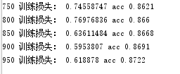
                print(i,"训练损失：",trainloss,'acc',test_acc)

十一、神经网络构建

"""mnist.py""""
import math

import tensorflow as tf

# The MNIST dataset has 10 classes, representing the digits 0 through 9.
NUM_CLASSES = 10

# The MNIST images are always 28x28 pixels.
IMAGE_SIZE = 28
IMAGE_PIXELS = IMAGE_SIZE * IMAGE_SIZE
batch_size = 50  # 每个批次的样本数量
hidden1_units = 20  # 第一个隐藏层神经元个数
hidden2_units = 15  # 第二个隐藏层神经元个数
learning_rate=0.1 #优化器的学习率

# 输入张量
images_placeholder = tf.compat.v1.placeholder(tf.float32, shape=(batch_size, IMAGE_PIXELS))
labels_placeholder = tf.compat.v1.placeholder(tf.int32, shape=(batch_size))


# 前向计算
def inference(images, hidden1_units, hidden2_units):
    """Build the MNIST model up to where it may be used for inference.
    Args:
      images: Images placeholder, from inputs().
      hidden1_units: Size of the first hidden layer.
      hidden2_units: Size of the second hidden layer.
    Returns:
      softmax_linear: Output tensor with the computed logits.
    """
    # Hidden 1
    with tf.compat.v1.name_scope('hidden1'):
        weights = tf.Variable(tf.random.truncated_normal([IMAGE_PIXELS, hidden1_units],
                stddev=1.0 / math.sqrt(float(IMAGE_PIXELS))), name='weights')
        biases = tf.Variable(tf.zeros([hidden1_units]),name='biases')
        hidden1 = tf.nn.relu(tf.matmul(images, weights) + biases)
    # Hidden 2
    with tf.compat.v1.name_scope('hidden2'):
        weights = tf.Variable(tf.random.truncated_normal( [hidden1_units, hidden2_units],
                stddev=1.0 / math.sqrt(float(hidden1_units))), name='weights')
        biases = tf.Variable(tf.zeros([hidden2_units]),name='biases')
        hidden2 = tf.nn.relu(tf.matmul(hidden1, weights) + biases)
    # Linear
    with tf.compat.v1.name_scope('softmax_linear'):
        weights = tf.Variable(tf.random.truncated_normal([hidden2_units, NUM_CLASSES],
                stddev=1.0 / math.sqrt(float(hidden2_units))), name='weights')
        biases = tf.Variable(tf.zeros([NUM_CLASSES]),name='biases')
        logits = tf.matmul(hidden2, weights) + biases
    return logits

# 定义损失函数
def loss(logits, labels):
  """Calculates the loss from the logits and the labels.
  Args:
    logits: Logits tensor, float - [batch_size, NUM_CLASSES].
    labels: Labels tensor, int32 - [batch_size].
  Returns:
    loss: Loss tensor of type float.
  """
  labels = tf.cast(labels, dtype=tf.int64)#将labels转为int64
  return tf.compat.v1.losses.sparse_softmax_cross_entropy(labels=labels, logits=logits)#交叉熵损失

#定义train字图
def training(loss, learning_rate):
  optimizer = tf.compat.v1.train.GradientDescentOptimizer(learning_rate)
  train_op = optimizer.minimize(loss)
  return train_op

# 评估
def evaluation(logits, labels):
  """Evaluate the quality of the logits at predicting the label.
  Args:
    logits: Logits tensor, float - [batch_size, NUM_CLASSES].
    labels: Labels tensor, int32 - [batch_size], with values in the
      range [0, NUM_CLASSES).
  Returns:
    A scalar int32 tensor with the number of examples (out of batch_size)
    that were predicted correctly.
  """
  # For a classifier model, we can use the in_top_k Op.
  # It returns a bool tensor with shape [batch_size] that is true for
  # the examples where the label is in the top k (here k=1)
  # of all logits for that example.
  correct = tf.nn.in_top_k(predictions=logits, targets=labels, k=1) #布尔
  # Return the number of true entries.
  return tf.reduce_sum(input_tensor=tf.cast(correct, tf.int32))

#nn_logits=inference(images_placeholder, hidden1_units, hidden2_units)
#nn_loss=loss(logits=nn_logits,labels=labels_placeholder)
#train_on_batch=training(loss=nn_loss, learning_rate=learning_rate)
#correct_count=evaluation(logits=nn_logits,labels=labels_placeholder)


# 计算图可视化，写入tensorboard
#writer = tf.summary.FileWriter("./logs", tf.get_default_graph())
#writer.close()

argparse.ArgumentParser()用法解析

运行计算图

"""full_connecttd_feed.py"""
import time
import numpy as np
import tensorflow as tf
from MY_MNIST import nn_mnist
from tensorflow.examples.tutorials.mnist import input_data

print('开始读入数据')
mnist = input_data.read_data_sets(r"E:\tensorflow_study\MNIST\MNIST_DATA", one_hot=True)
print('数据读取完毕')


"""导入数据"""
# The MNIST dataset has 10 classes, representing the digits 0 through 9.
NUM_CLASSES = 10
IMAGE_SIZE = 28
IMAGE_PIXELS = IMAGE_SIZE * IMAGE_SIZE
batch_size = 100  # 每个批次的样本数量
hidden1_units = 20  # 第一个隐藏层神经元个数
hidden2_units = 15  # 第二个隐藏层神经元个数
learning_rate=0.1 #优化器的学习率

"""构建并可视化计算图"""
"""初始化节点，运行计算图"""
def creat_graph():
    images_placeholder=nn_mnist.images_placeholder
    labels_placeholder=nn_mnist.labels_placeholder
    nn_logits=nn_mnist.inference(images_placeholder, hidden1_units, hidden2_units)
    nn_loss=nn_mnist.loss(logits=nn_logits,labels=labels_placeholder)
    train_on_batch=nn_mnist.training(loss=nn_loss, learning_rate=learning_rate)
    correct_count=nn_mnist.evaluation(logits=nn_logits,labels=labels_placeholder)
    init = tf.global_variables_initializer()
    # 计算图可视化，写入tensorboard
    writer = tf.summary.FileWriter(r"E:\tensorflow_study\MY_MNIST\mnist_log", tf.get_default_graph())
    writer.close()
    with tf.Session() as sees:
        sees.run(init)
        # 开始按批次训练，共训练1000批次，每批次100个数据

        for i in range(2001):
            batch_xs, batch_y = mnist.train.next_batch(batch_size)
            batch_ys=np.argmax(batch_y, axis=1)
            _, trainloss = sees.run([train_on_batch, nn_loss], feed_dict={images_placeholder: batch_xs, labels_placeholder: batch_ys})
            if i % 100 == 0:
                print(i, "训练损失：", trainloss)
            if i % 500 == 0:
                test_acc = sees.run(correct_count, feed_dict={labels_placeholder: np.argmax(mnist.test.labels,axis=1), images_placeholder: mnist.test.images})
                print( 'acc_test', test_acc/(np.argmax(mnist.test.labels,axis=1).size))


if __name__ == '__main__':
    creat_graph()

*补充：Summary汇总标量

在计算图的构建里的训练过程——优化器部分加入

# 定义train字图
def training(loss, learning_rate):
    """********"""
    """测试summary功能"""
    """********"""
#1、写入需要汇总的
    with tf.name_scope('Scalar_Summaries'):
        tf.summary.scalar('loss', loss)
        tf.summary.scalar('learning_rate', learning_rate)
    optimizer = tf.compat.v1.train.GradientDescentOptimizer(learning_rate)
#2、global_step
    global_step = tf.Variable(0, name='global_step', trainable=False)
    train_op = optimizer.minimize(loss, global_step)
    return train_op

在主函数运行，计算图运行部分加入

#1、汇总summary
    summaries=tf.summary.merge_all()

    """计算图可视化，写入tensorboard"""
#2、tf.summary.FileWriter
    writer = tf.summary.FileWriter(r"E:\tensorflow_study\MY_MNIST\mnist_log", tf.get_default_graph())
    #writer.close()

    with tf.Session() as sees:
        sees.run(init)
        # 开始按批次训练，共训练1000批次，每批次100个数据

        for i in range(1001):
            batch_xs, batch_y = mnist.train.next_batch(batch_size)
            batch_ys=np.argmax(batch_y, axis=1)
            #总数据集
            data=feed_dict={labels_placeholder: np.argmax(mnist.test.labels,axis=1), images_placeholder: mnist.test.images}
            _, trainloss = sees.run([train_on_batch, nn_loss], feed_dict={images_placeholder: batch_xs, labels_placeholder: batch_ys})
            if i % 100 == 0:
                print(i, "训练损失：", trainloss)
 #3、
                """"********"""
                """每隔100次汇总一下summary"""
                """"********"""
                summaries_merge=sees.run(summaries,feed_dict={images_placeholder: batch_xs, labels_placeholder: batch_ys})
                writer.add_summary(summaries_merge, i)
                writer.flush()

*补充：summary保存点文件

 # Create a saver for writing training checkpoints.
 #1、

                 """"********"""
                 """"在运行session前加入"""
                """"********"""
    saver = tf.compat.v1.train.Saver()

    with tf.Session() as sees:
        sees.run(init)
        # 开始按批次训练，共训练1000批次，每批次100个数据

        for i in range(1001):
            batch_xs, batch_y = mnist.train.next_batch(batch_size)
            batch_ys=np.argmax(batch_y, axis=1)
            #总数据集
            data=feed_dict={labels_placeholder: np.argmax(mnist.test.labels,axis=1), images_placeholder: mnist.test.images}
            _, trainloss = sees.run([train_on_batch, nn_loss], feed_dict={images_placeholder: batch_xs, labels_placeholder: batch_ys})
            if i % 100 == 0:
                print(i, "训练损失：", trainloss)



                summaries_merge=sees.run(summaries,feed_dict={images_placeholder: batch_xs, labels_placeholder: batch_ys})
                writer.add_summary(summaries_merge, i)
                writer.flush()

            if i % 1000 == 0:
#2、
                 """"********"""
                 """"保存到事件日志同名文件夹下，注意加后缀model.ckpt"""
                """"********"""

                saver.save(sees,r'E:\tensorflow_study\MY_MNIST\mnist_log/model.ckpt',i)

                test_acc = sees.run(correct_count, feed_dict=data)
                print( 'acc_test', test_acc/(np.argmax(mnist.test.labels,axis=1).size))

十二、summary(直方图，图片，均值，方差)

from __future__ import absolute_import
from __future__ import division
from __future__ import print_function

import argparse
import os
import sys

import tensorflow as tf

from tensorflow.examples.tutorials.mnist import input_data

FLAGS = None


# 汇总函数，对一个张量进行全面绘总（均值、标准差、最大最小值、直方图）
def variable_summaries(var):
    """Attach a lot of summaries to a Tensor (for TensorBoard visualization)."""
    with tf.compat.v1.name_scope('summaries'):
      mean = tf.reduce_mean(input_tensor=var)
      tf.compat.v1.summary.scalar('mean', mean)
      with tf.compat.v1.name_scope('stddev'):
        stddev = tf.sqrt(tf.reduce_mean(input_tensor=tf.square(var - mean)))
      tf.compat.v1.summary.scalar('stddev', stddev)
      tf.compat.v1.summary.scalar('max', tf.reduce_max(input_tensor=var))
      tf.compat.v1.summary.scalar('min', tf.reduce_min(input_tensor=var))
      tf.compat.v1.summary.histogram('histogram', var)


# 权值初始化
def weight_variable(shape):
    """Create a weight variable with appropriate initialization."""
    initial = tf.random.truncated_normal(shape, stddev=0.1)
    return tf.Variable(initial)


# 偏置初始化
def bias_variable(shape):
    """Create a bias variable with appropriate initialization."""
    initial = tf.constant(0.1, shape=shape)
    return tf.Variable(initial)


# 隐藏层函数构建
def nn_layer(input_tensor, input_dim, output_dim, layer_name, act=tf.nn.relu):
    with tf.compat.v1.name_scope(layer_name):
        # This Variable will hold the state of the weights for the layer
        with tf.compat.v1.name_scope('weights'):
            weights = weight_variable([input_dim, output_dim])
            variable_summaries(weights)
        with tf.compat.v1.name_scope('biases'):
            biases = bias_variable([output_dim])
            variable_summaries(biases)
        with tf.compat.v1.name_scope('Wx_plus_b'):
            preactivate = tf.matmul(input_tensor, weights) + biases
            tf.compat.v1.summary.histogram('pre_activations', preactivate)
        activations = act(preactivate, name='activation')
        tf.compat.v1.summary.histogram('activations', activations)
        return activations



def train():
    # Input placeholders
    with tf.compat.v1.name_scope('input'):
        x = tf.compat.v1.placeholder(tf.float32, [None, 784], name='x-input')
        y_ = tf.compat.v1.placeholder(tf.int64, [None], name='y-input')

    with tf.compat.v1.name_scope('input_reshape'):
        image_shaped_input = tf.reshape(x, [-1, 28, 28, 1])
        tf.compat.v1.summary.image('input', image_shaped_input, 10)


    # 隐藏层1
    hidden1 = nn_layer(x, 784, 500, 'layer1')

    # drop-out层
    with tf.compat.v1.name_scope('dropout'):
        keep_prob = tf.compat.v1.placeholder(tf.float32)
        tf.compat.v1.summary.scalar('dropout_keep_probability', keep_prob)
        dropped = tf.nn.dropout(hidden1, rate=(1 - keep_prob))

        # 隐藏层2
    logits = nn_layer(dropped, 500, 10, 'layer2', act=tf.identity)

    # 交叉熵损失
    with tf.compat.v1.name_scope('cross_entropy'):
        # tf.reduce_mean(-tf.reduce_sum(y_ * tf.math.log(tf.softmax(y)),reduction_indices=[1]))
        with tf.compat.v1.name_scope('total'):
            cross_entropy = tf.compat.v1.losses.sparse_softmax_cross_entropy(labels=y_, logits=logits)
            tf.compat.v1.summary.scalar('cross_entropy', cross_entropy)

    # 　训练节点
    with tf.compat.v1.name_scope('train'):
        train_step = tf.compat.v1.train.AdamOptimizer(FLAGS.learning_rate).minimize(cross_entropy)

    # 评估准确率
    with tf.compat.v1.name_scope('accuracy'):
        with tf.compat.v1.name_scope('correct_prediction'):
            correct_prediction = tf.equal(tf.argmax(input=logits, axis=1), y_)
        with tf.compat.v1.name_scope('accuracy'):
            accuracy = tf.reduce_mean(input_tensor=tf.cast(correct_prediction,tf.float32))
    tf.compat.v1.summary.scalar('accuracy', accuracy)


    # Import data
    mnist = input_data.read_data_sets(FLAGS.data_dir, fake_data=FLAGS.fake_data)

    def feed_dict(train):
        """Make a TensorFlow feed_dict: maps data onto Tensor placeholders."""
        if train or FLAGS.fake_data:
            xs, ys = mnist.train.next_batch(100, fake_data=FLAGS.fake_data)
            k = FLAGS.dropout
        else:
            xs, ys = mnist.test.images, mnist.test.labels
            k = 1.0
        return {x: xs, y_: ys, keep_prob: k}



    # 声明一个会话
    sess = tf.compat.v1.InteractiveSession()

    merged = tf.compat.v1.summary.merge_all()
    train_writer = tf.compat.v1.summary.FileWriter(r'E:\tensorflow_study\MY_MNIST\mnist_log\train',
                                                   sess.graph)
    test_writer = tf.compat.v1.summary.FileWriter(r'E:\tensorflow_study\MY_MNIST\mnist_log\test')


 # 全局变量初始化
    tf.global_variables_initializer().run()

    # 开始迭代训练
    for i in range(FLAGS.max_steps):

        if i % 20 == 0:
            summary, _, train_loss = sess.run([merged, train_step, cross_entropy], feed_dict=feed_dict(True))
            print("step:", i, "train_loss:", train_loss)
            train_writer.add_summary(summary, i)
        # 评估测试集
        if i%100==0:
            summary,acc=sess.run([merged,accuracy],feed_dict=feed_dict(False))
            print("step:",i,"acc_test:",acc)
            test_writer.add_summary(summary, i)

    # # 计算图可视化，写入tensorboard
    # writer = tf.summary.FileWriter(r'E:\tensorflow_study\MY_MNIST\mnist_log', tf.get_default_graph())
    # writer.close()


def main(_):
    # 创建存放事件日志和模型检查点的文件夹
    if tf.io.gfile.exists(FLAGS.log_dir):
        tf.io.gfile.rmtree(FLAGS.log_dir)
    tf.io.gfile.makedirs(FLAGS.log_dir)
    # 启动训练过程
    with tf.Graph().as_default():
        train()


if __name__ == '__main__':
    parser = argparse.ArgumentParser()
    parser.add_argument('--fake_data', nargs='?', const=True, type=bool,
                        default=False,
                        help='If true, uses fake data for unit testing.')
    parser.add_argument('--max_steps', type=int, default=1000,
                        help='Number of steps to run trainer.')
    parser.add_argument('--learning_rate', type=float, default=0.001,
                        help='Initial learning rate')
    parser.add_argument('--dropout', type=float, default=0.9,
                        help='Keep probability for training dropout.')
    parser.add_argument(
        '--data_dir',
        type=str,
        default=r'E:\tensorflow_study\MY_MNIST\MNIST_DATA',
        help='Directory to put the input data.'
    )
    parser.add_argument(
        '--log_dir',
        type=str,
        default=r'E:\tensorflow_study\MY_MNIST\logss',
        help='Directory to put the log data.'
    )
    FLAGS, unparsed = parser.parse_known_args()
    main([sys.argv[0]] + unparsed)

十三、ArgumentParser，tf.ConfigProto() 和 XLA JIT编译，RunOptions和RunMetadata和Timeline

mnist_softmax_xla分析