吴恩达——机器学习ex5(Regularized Linear Regression and Bias v.s. Variance)

1.1 Visualizing the dataset

import matplotlib.pyplot as plt
import scipy.io


data = scipy.io.loadmat('data/ex5data1.mat')
# print(data.keys())
'''绘制training data'''
a = data['X']
b = data['y']
plt.scatter(a, b, c='red', marker='x', s=20)
plt.xlabel('Change in water level (x)')
plt.ylabel('Water flowing out of the dam (y)')
plt.show()

1.2/3 Regularized linear regression cost function and gradient

这里的向量化写法和ex3的logistic regression的写法类似，这里略作修改，当作对ex2里面笨笨的写法的修正。

"""linearRegCostFunction.py函数"""
import numpy as np

def g(z):
    h = 1./(1+np.exp(-z))
    return h

"""加上正则化的代价函数及其偏导数"""
def linearRegCostFunction(X, Y, theta, lmda):
    m = X.shape[0]
    n = X.shape[1]
    # fmin输出的theta是(n,)要正确运算，需reshpe 成(n,1)               )
    theta = theta.reshape(n, 1)
    h = X.dot(theta)
    Y = Y.reshape(m, 1)

    # 代价函数
    J = (h - Y).T.dot(h - Y)/2/m + (theta[1:].T.dot(theta[1:]))*lmda/2/m
    # 代价函数的导数
    J_d = X.T.dot(h-Y)/m
    J_d[0]=J_d[0]
    J_d[1:] = J_d[1:] + lmda * theta[1:]/m
    # 由于fmin 输入的函数必得是（n,）的形式，故需要将J_dreshape成（n,）的形式
    J_d = J_d.reshape(J_d.size)
    return J, J_d




"""主函数调用"""
'''编写代价函数'''
# 为X1增加一列，构成(12, 2)的输入样本
X = np.hstack((np.ones((X1.shape[0])).reshape(X1.shape[0], 1), X1))
theta_init = np.ones((2, 1))
lmda = 1
J, J_d = linearRegCostFunction(X, y, theta_init, lmda)
print('预计代价应为303.993', J)
print('预计梯度应为[-15.30; 598.250]', J_d)

1.4 Fitting linear regression

用线性回归（最优化）拟合样本

import scipy.optimize as opt
from linearRegCostFunction import linearRegCostFunction


def line_trainLinearReg(theta_init, X, y, lmda):
    def cost_func(t):
        return linearRegCostFunction(X, y, t, lmda)[0]

    def grad_func(t):
        return linearRegCostFunction(X, y, t, lmda)[1]

    # 使用opt.fmin_bfgs()来获得最优解
    theta, cost, *unused = opt.fmin_bfgs(f=cost_func, fprime=grad_func, x0=theta_init, maxiter=400, full_output=True, disp=False)
    return theta



"""主函数调用"""
'''用线性函数拟合样本'''
n = X.shape[1]
m = X.shape[0]
# fmin输出的theta是(n,)要正确运算，需reshpe 成(n,1)
theta = line_trainLinearReg(theta_init, X, y, lmda)
theta = theta.reshape(n, 1)
a = [-50, 40]
b = [theta[0]-50*theta[1], theta[0]+40*theta[1]]
plt.figure(0)
plt.plot(a, b, 'b-', lw=1)  # 绘制直线图

2 Bias-variance

高偏差欠拟合，高方差过拟合。

2.1 Learning curves

通过绘制训练集误差（training_set）和验证交叉集误差(cross validation error)随样本长度m的变化情况，来判断是否欠拟合或过拟合。
即m（i=0:m）逐渐增加的过程中，求出每个m对应的theta，然后求m个样本的训练集误差和交叉验证集误差。

注意：Speci cally, for a training set size of i, you should use the rst i examples (i.e., X(1:i,:)and y(1:i)).
训练误差：（注意没有正则化项）

从上图可知，当样本增加，训练集和交叉验证集误差都很大，欠拟合。应该增加特征数或多项式次数来改善。

import numpy as np
from line_trainLinearReg import line_trainLinearReg
from linearRegCostFunction import linearRegCostFunction
def learningCurve(X, Xval, y, yval, theta_init, lmda):
    m = X.shape[0]
    J_test = np.zeros(m)
    J_val = np.zeros(m)
    for i in range(m):
        X_A = X[:i+1, :] # 新样本长度
        y_A = y[:i+1]
        theta = line_trainLinearReg(theta_init, X_A, y_A, lmda)
        J_test[i] = linearRegCostFunction(X_A, y_A, theta, lmda)[2]
        J_val[i] = linearRegCostFunction(Xval, yval, theta, lmda)[2]
    return J_test, J_val


'''主函数调用'''
'''绘制误差曲线，观察是否过拟合欠拟合'''
J_train, J_val = learningCurve(X, Xval, y, yval, theta_init, lmda)
plt.figure(1)
plt.plot(range(m),J_train, range(m),J_val)
plt.title('Learning curve for linear regression')
plt.xlabel('m')
plt.ylabel('Error')
plt.show()

3 Polynomial regression

首先生成下面一组新样本

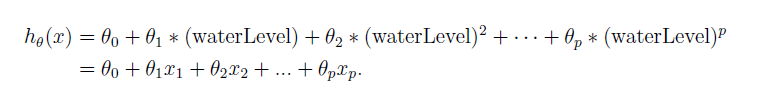
从下式中可以看出，我们单纯的把多项式高阶项看作特征，故多项式回归其本质是多特征的线性回归。

import numpy as np

def polyFeatures(X1, p):
    for i in range(2, p+1):
        X1 = np.hstack((X1, (X1[:,0].reshape(3,1))**i))
    return X1

"""应用到训练集、测试集、交叉验证集"""
'''增加特征数'''
X1_pol = polyFeatures(X1, 3)
Xtest_pol = polyFeatures(Xtest, 3)
Xval_pol = polyFeatures(Xval, 3)
X_pol = np.hstack((np.ones((X1_pol.shape[0])).reshape(X1_pol.shape[0], 1), X1_pol))
Xtest_pol = np.hstack((np.ones((Xtest_pol.shape[0])).reshape(Xtest_pol.shape[0], 1), Xtest_pol))
Xval_pol = np.hstack((np.ones((Xval_pol.shape[0])).reshape(Xval_pol.shape[0], 1), Xval_pol))

3.1 Learning Polynomial Regression

1. 首先注意，由于出现了$x^p$，因而特征可能差异较大，我们首先进行特征归一化，这在ex1里面已经提到过（注意不要对偏置项（第一列全为1）进行归一化。）
2. 然后进行线性回归学习theta，
3. 代价函数学习梯度和代价
4. 绘制拟合曲线，描点连线，取很多个x，归一化，计算对应的yfit，描点。

import numpy as np
from polyFeatures import polyFeatures
# 输入横坐标范围，计算出拟合曲线在每一点的取值
def plotFit(min_x,max_x,mu,sigma,theta,p):
   x = np.arange(min_x-10,max_x+10, 0.05)
   x = x.reshape(x.size, 1)

   X_poly = polyFeatures(x, p)
   X_poly -= mu
   X_poly /= sigma
   X_poly = np.column_stack((np.ones(x.size), X_poly))

   Y_fit = X_poly.dot(theta)

   return x, Y_fit


"""主函数"""
"""线性回归最优化学习参数theta"""
theta_pol_init = np.zeros((9, 1))
lmda = 0
theta_pol = line_trainLinearReg(theta_pol_init, X_pol, y, lmda)
x, yfit = plotFit(min(X1), max(X1), X_pol_mean, X_pol_std, theta_pol, 8)

'''用线性函数拟合样本'''
plt.figure(2)
plt.plot(x, yfit, 'b-', lw=1)  # 绘制直线图
plt.scatter(X1, y, c='red', marker='x', s=20)
plt.xlabel('Change in water level (x)')
plt.ylabel('Water flowing out of the dam (y)')
plt.show()

'''绘制误差曲线，观察是否过拟合欠拟合'''
J_train_pol, J_val_pol = learningCurve(X_pol, Xval_pol, y, yval, theta_pol_init, lmda)
plt.figure(3)
plt.plot(range(m),J_train_pol, range(m),J_val_pol)
plt.title('Learning curve for polynomial regression')
plt.xlabel('m')
plt.ylabel('Error')
plt.show()

从上图曲线中可以看出，低偏差，高方差，过拟合。

3.2 Optional (ungraded) exercise: Adjusting the regularization parameter

正则化系数$lmda=1$时，由下图可以看出偏差和方差都很小，此时拟合效果较好。

正则化系数$lmda=100$时，此时拟合效果很差。

3.3 Selecting lmda using a cross validation set

You should try in the following range: [0; 0:001; 0:003; 0:01; 0:03; 0:1; 0:3; 1; 3; 10g]，绘制lmda和误差曲线

import numpy as np
from linearRegCostFunction import linearRegCostFunction
from line_trainLinearReg import line_trainLinearReg


def validationCurve(theta_init, X, X_val, y, y_val):
    lmdaa = np.array([0., 0.001, 0.003, 0.01, 0.03, 0.1, 0.3, 1, 3, 10])
    error_train = np.zeros(lmdaa.size)
    error_val = np.zeros(lmdaa.size)
    for i in range(lmdaa.size):
        lmd = lmdaa[i]
        theta = line_trainLinearReg(theta_init, X, y, lmd)
        error_train[i],_ ,_ = linearRegCostFunction(X, y, theta, lmd)
        error_val[i],_ ,_ = linearRegCostFunction(X_val, y_val, theta, lmd)
    return error_train, error_val


"""主程序"""
"""自动选择lmda"""
lmda = np.array([0,0.001,0.003, 0.01,0.03, 0.1, 0.3, 1, 3, 10])
J_train_pol_l, J_val_pol_l = validationCurve(theta_pol_init, X_pol, Xtest_pol, y, ytest)
plt.figure(4)
plt.plot(lmda,J_train_pol_l, lmda,J_val_pol_l)
plt.title('Learning lmda for polynomial regression')
plt.xlabel('lmda')
plt.ylabel('Error')
plt.show()

3.4 Optional (ungraded) exercise: Computing test set error

lmda = 3
theta = line_trainLinearReg(theta_pol_init,  X_pol, y, lmda)
J = linearRegCostFunction(Xval_pol, yval, theta, lmda)[0]
print('J Suppose to be 3.8599', J)

代码已上传至：https://github.com/hellobigorange/my_own_machineLearning/tree/master/my_ex5