深度学习：完全理解反向传播算法（二）

---

1. 前言

前情提要：
《深度学习：完全理解反向传播算法（一）》

上文已经推导了反向传播的基本公式，如下：

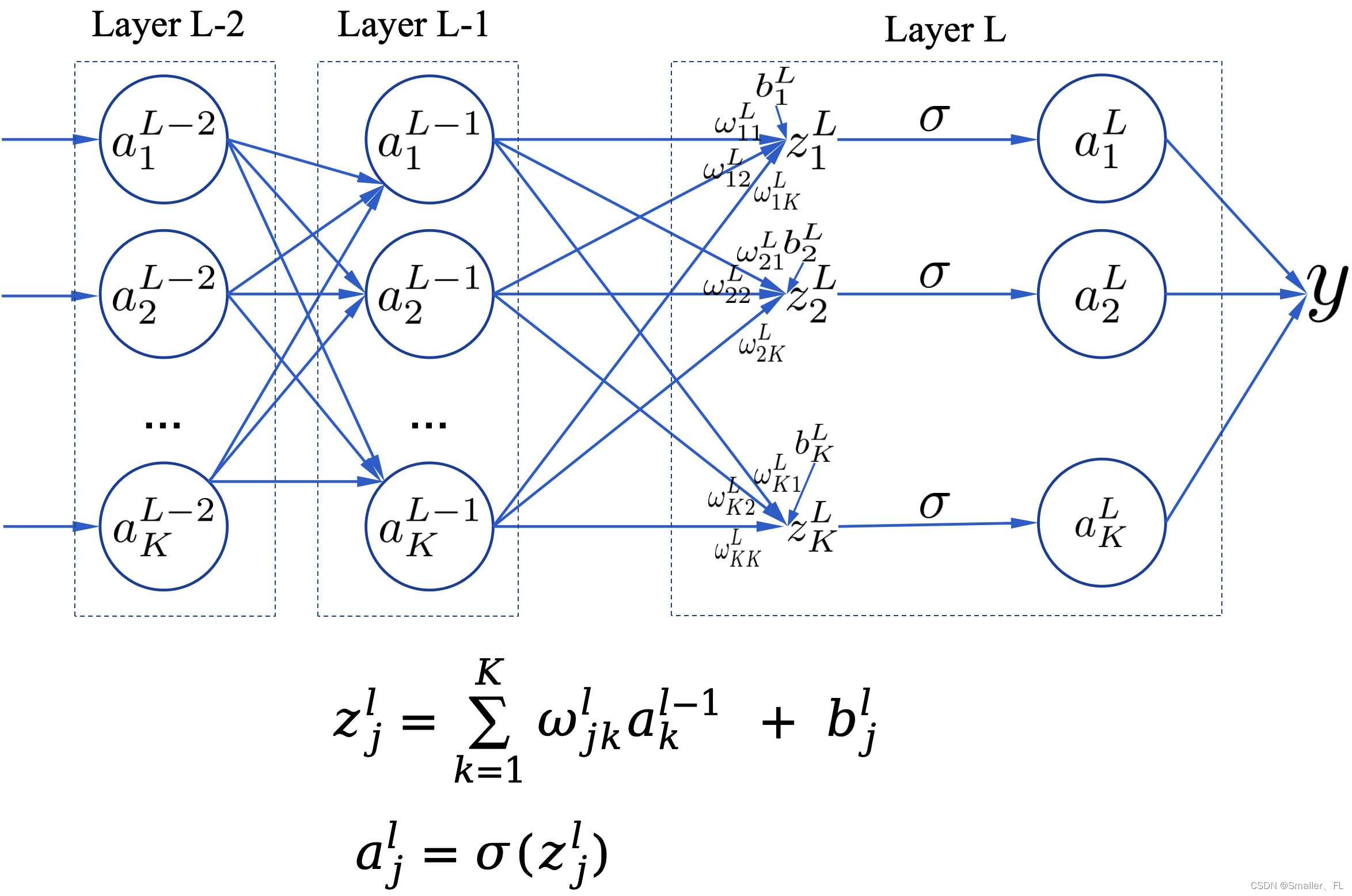
损失函数：
$$C=\frac{1}{2}||y-a^L|{|}^2=\frac{1}{2}\sum _{k=1}^K(y_k-a_k^L{)}^2$$

损失函数对 $a_j^L$ 的偏导数：
$$\frac{\partial C}{\partial a_j^L}=a_j^L-y_j$$
反向传播的四个基本方程式：
$${\delta }^L={\nabla }_{a}C\odot {\sigma }^{\prime }(z^L)$$
$${\delta }_j^l=(({\omega }^{l+1}{)}^T{\delta }^{l+1})\odot {\sigma }^{\prime }(z^l)$$
$$\frac{\partial C}{\partial b_j^l}={\delta }_j^l$$
$$\frac{\partial C}{\partial {\omega }_{jk}^l}={\delta }_j^l{a}_k^{l-1}$$

本文主要介绍反向传播的算法流程！

2. 反向传播算法流程

2.1 伪代码

在实践中，通常将反向传播与随机梯度下降等学习算法结合起来，其中我们计算许多训练示例的梯度。给定一个由 m 个训练样例组成的小批次（mini-batch）数据，以下算法基于该小批次应用梯度下降学习步骤:
1. 输入一系列训练数据
2. 对于每个训练批次 $x$，计算如下内容:

• 前向传播： For each $l=2,3,..,L$ 计算 $z^{x,l}={\omega }^l{a}^{x,l-1}+b^l$ 以及 $a^{x,l}=\sigma (z^{x,l})$
• 输出误差： ${\delta }^{x,L}={\nabla }_a{C}_x\odot {\sigma }^{\prime }(z^{x,L})$
• 反向传播误差： For each $l=L-1,L-2,..,2$ 计算 ${\delta }_j^{x,l}=(({\omega }^{l+1}{)}^T{\delta }^{x,l+1})\odot {\sigma }^{\prime }(z^{x,l})$

3. 梯度下降： For each $l=L,L-1,..,2$，更新权重 ${\omega }^l=w^l-\frac{\eta }{m}{\sum }_x{\delta }^{x,l}(a^{x,l-1}{)}^T$ 以及偏置 $b^l=b^l-\frac{\eta }{m}{\sum }_x{\delta }^{x,l}$

解释下伪代码里的梯度下降：

1. $\eta$ 就是常听到的学习率，用于给权重和偏置的变动乘于一个调整的系数
2. 权重 $\omega$ 为什么要减去 ${\sum }_x{\delta }^{x,l}(a^{x,l-1}{)}^T$？首先一个小批次是 $x$，我们要减去所有批次的结果，那么自然有一个求和 ${\sum }_x$。其次，误差对于权重的求导 $\frac{\partial C}{\partial {\omega }_{jk}^l}={\delta }_j^l{a}_k^{l-1}$，也就是说权重需要反向变动以达到减少误差的效果，因此需要减去 ${\sum }_x{\delta }^{x,l}(a^{x,l-1}{)}^T$
3. 对于偏置，解释同上

2.2 实际代码

在 《How the backpropagation algorithm works》 文章中，给出了 MNIST 手写数字识别的反向传播的代码。MNIST 在 CV 领域是一个经典的 hello world 项目。MNIST 项目代码：

git clone https://github.com/mnielsen/neural-networks-and-deep-learning.git

其中的代码：

class Network(object)
...
    def update_mini_batch(self, mini_batch, eta, lmbda, n):
        """Update the network's weights and biases by applying gradient
        descent using backpropagation to a single mini batch.  The
        ``mini_batch`` is a list of tuples ``(x, y)``, ``eta`` is the
        learning rate, ``lmbda`` is the regularization parameter, and
        ``n`` is the total size of the training data set.

        """
        nabla_b = [np.zeros(b.shape) for b in self.biases]
        nabla_w = [np.zeros(w.shape) for w in self.weights]
        for x, y in mini_batch:
        	# 对于每一个批次，计算反向传播需要调整的结果，其中包含计算伪代码的 “反向传播误差” 这一步骤
            delta_nabla_b, delta_nabla_w = self.backprop(x, y)
            nabla_b = [nb+dnb for nb, dnb in zip(nabla_b, delta_nabla_b)]
            nabla_w = [nw+dnw for nw, dnw in zip(nabla_w, delta_nabla_w)]
        # 对应伪代码的 “梯度下降” 这一步骤
        # weight这里增加一个lmbda参数，用于降低过拟合
        self.weights = [(1-eta*(lmbda/n))*w-(eta/len(mini_batch))*nw
                        for w, nw in zip(self.weights, nabla_w)]
        self.biases = [b-(eta/len(mini_batch))*nb
                       for b, nb in zip(self.biases, nabla_b)]

关键的是 backprop，即反向传播代码：

    def backprop(self, x, y):
        """Return a tuple ``(nabla_b, nabla_w)`` representing the
        gradient for the cost function C_x.  ``nabla_b`` and
        ``nabla_w`` are layer-by-layer lists of numpy arrays, similar
        to ``self.biases`` and ``self.weights``."""
        nabla_b = [np.zeros(b.shape) for b in self.biases]
        nabla_w = [np.zeros(w.shape) for w in self.weights]
        # 这里先前向计算一遍，对应于伪代码的 “前向传播” 这一步骤
        activation = x
        activations = [x] # list to store all the activations, layer by layer
        zs = [] # list to store all the z vectors, layer by layer
        for b, w in zip(self.biases, self.weights):
            z = np.dot(w, activation)+b
            zs.append(z)
            activation = sigmoid(z)
            activations.append(activation)
        # backward pass
        # 这里计算输出误差 aL - y
        delta = (self.cost).delta(zs[-1], activations[-1], y)
        nabla_b[-1] = delta
        nabla_w[-1] = np.dot(delta, activations[-2].transpose())
        # Note that the variable l in the loop below is used a little
        # differently to the notation in Chapter 2 of the book.  Here,
        # l = 1 means the last layer of neurons, l = 2 is the
        # second-last layer, and so on.  It's a renumbering of the
        # scheme in the book, used here to take advantage of the fact
        # that Python can use negative indices in lists.
        # 对应于伪代码的 “反向传播误差” 这一步骤
        for l in xrange(2, self.num_layers):
            z = zs[-l]
            # sp：对 z 求导
            sp = sigmoid_prime(z)
            # 对应于四个基础方程的第二个！
            delta = np.dot(self.weights[-l+1].transpose(), delta) * sp
            # 对应于四个基础方程的第三个！
            nabla_b[-l] = delta
            # 对应于四个基础方程的第四个！
            nabla_w[-l] = np.dot(delta, activations[-l-1].transpose())
        return (nabla_b, nabla_w)

代码解释都在上面的中文注释中了，核心就是四个基本方程式。

至此，反向传播的主要内容完结，希望有所收获～

3. 参考

《Learning representations by back-propagating errors》
《How the backpropagation algorithm works》

欢迎关注本人，我是喜欢搞事的程序猿； 一起进步，一起学习；

也欢迎关注我的wx公众号：一个比特定乾坤