ARIMA模型（p,d,q）参数确定（python）

参数d:

ARIMA 模型对时间序列的要求是平稳型。因此，当你得到一个非平稳的时间序列时，首先要做的即是做时间序列的差分，直到得到一个平稳时间序列。如果你对时间序列做d次差分才能得到一个平稳序列，那么可以使用ARIMA(p,d,q)模型，其中d是差分次数。

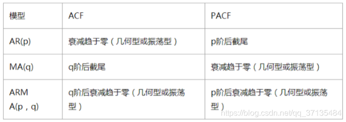
模型的参数p和q由ACF和PACF确定

如下表格

statsmodels介绍

statsmodels（http://www.statsmodels.org）是一个Python库，用于拟合多种统计模型，执行统计测试以及数据探索和可视化。statsmodels包含更多的“经典”频率学派统计方法，而贝叶斯方法和机器学习模型可在其他库中找到。
包含在statsmodels中的一些模型：

• 线性模型，广义线性模型和鲁棒线性模型
• 线性混合效应模型
• 方差分析（ANOVA）方法
• 时间序列过程和状态空间模型
• 广义的矩量法

我们使用其中的时间序列相关函数进行模型的构建。数据为历年美国消费者信心指数数据，代码如下：

%load_ext autoreload
%autoreload 2
%matplotlib inline
%config InlineBackend.figure_format='retina'
import pandas as pd
import numpy as np
import statsmodels.api as sm
import statsmodels.formula.api as smf
import statsmodels.tsa.api as smt
#Display and Plotting
import matplotlib.pylab as plt
import seaborn as sns
# pandas与numpy属性设置
pd.set_option('display.float_format',lambda x:'%.5f'%x)#pandas
np.set_printoptions(precision=5,suppress=True) #numpy
pd.set_option('display.max_columns',100)
pd.set_option('display.max_rows',100)
#seaborn.plotting style
sns.set(style='ticks',context='poster')

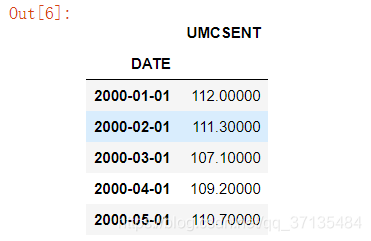
Sentiment='sentiment.csv'
Sentiment=pd.read_csv(Sentiment,index_col=0,parse_dates=[0])

Sentiment.head()

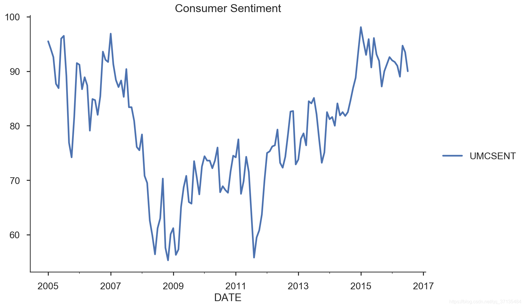
#选取时间断
sentiment_short=Sentiment.loc['2005':'2016']
sentiment_short.plot(figsize=(12,8))
plt.legend(bbox_to_anchor=(1.25,0.5))
plt.title('Consumer Sentiment')
sns.despine()

#help(sentiment_short['UMCSENT'].diff(1))
#函数diss()作用：https://blog.csdn.net/qq_32618817/article/details/80653841#
#https://blog.csdn.net/You_are_my_dream/article/details/700