机器学习实战-SVM算法-27

SVM算法-线性分类

import numpy as np
import matplotlib.pyplot as plt
from sklearn import svm

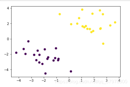
# 创建40个点
x_data = np.r_[np.random.randn(20, 2) - [2, 2], np.random.randn(20, 2) + [2, 2]]
y_data = [0]*20 +[1]*20

plt.scatter(x_data[:,0],x_data[:,1],c=y_data)
plt.show()

#fit the model
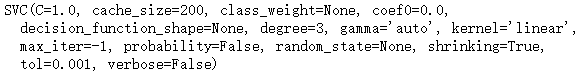
model = svm.SVC(kernel='linear')
model.fit(x_data, y_data)

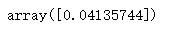
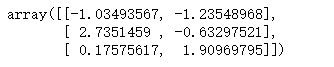
model.coef_

model.intercept_

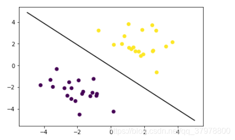
# 获取分离平面 

plt.scatter(x_data[:,0],x_data[:,1],c=y_data)
x_test = np.array([[-5],[5]])
d = -model.intercept_/model.coef_[0][1]
k = -model.coef_[0][0]/model.coef_[0][1]
y_test = d + k*x_test
plt.plot(x_test, y_test, 'k')
plt.show()

model.support_vectors_

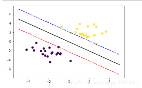
# 画出通过支持向量的分界线
b1 = model.support_vectors_[0]
y_down = k*x_test + (b1[1] - k*b1[0])
b2 = model.support_vectors_[-1]
y_up = k*x_test + (b2[1] - k*b2[0])

plt.scatter(x_data[:,0],x_data[:,1],c=y_data)
x_test = np.array([[-5],[5]])
d = -model.intercept_/model.coef_[0][1]
k = -model.coef_[0][0]/model.coef_[0][1]
y_test = d + k*x_test
plt.plot(x_test, y_test, 'k')
plt.plot(x_test, y_down, 'r--')
plt.plot(x_test, y_up, 'b--')
plt.show()

SVM算法-非线性分类

import matplotlib.pyplot as plt
import numpy as np
from sklearn.metrics import classification_report
from sklearn import svm

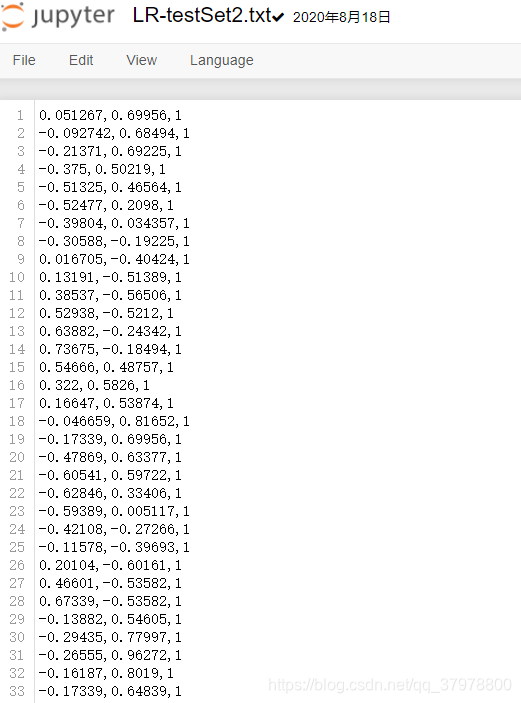
# 载入数据
data = np.genfromtxt("LR-testSet2.txt", delimiter=",")
x_data = data[:,:-1]
y_data = data[:,-1]
    
def plot():
    x0 = []
    x1 = []
    y0 = []
    y1 = []
    # 切分不同类别的数据
    for i in range(len(x_data)):
        if y_data[i]==0:
            x0.append(x_data[i,0])
            y0.append(x_data[i,1])
        else:
            x1.append(x_data[i,0])
            y1.append(x_data[i,1])

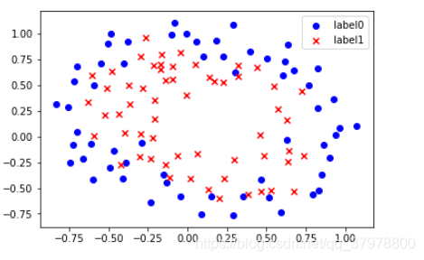
    # 画图
    scatter0 = plt.scatter(x0, y0, c='b', marker='o')
    scatter1 = plt.scatter(x1, y1, c='r', marker='x')
    #画图例
    plt.legend(handles=[scatter0,scatter1],labels=['label0','label1'],loc='best')
    
plot()
plt.show()

# fit the model
# C和gamma
# 'linear', 'poly', 'rbf', 'sigmoid'
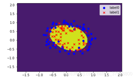
model = svm.SVC(kernel='rbf', C=2, gamma=1)
model.fit(x_data, y_data)

model.score(x_data,y_data)

# 获取数据值所在的范围
x_min, x_max = x_data[:, 0].min() - 1, x_data[:, 0].max() + 1
y_min, y_max = x_data[:, 1].min() - 1, x_data[:, 1].max() + 1

# 生成网格矩阵
xx, yy = np.meshgrid(np.arange(x_min, x_max, 0.02),
                     np.arange(y_min, y_max, 0.02))

z = model.predict(np.c_[xx.ravel(), yy.ravel()])# ravel与flatten类似，多维数据转一维。flatten不会改变原始数据，ravel会改变原始数据
z = z.reshape(xx.shape)

# 等高线图
cs = plt.contourf(xx, yy, z)
plot() 
plt.show()

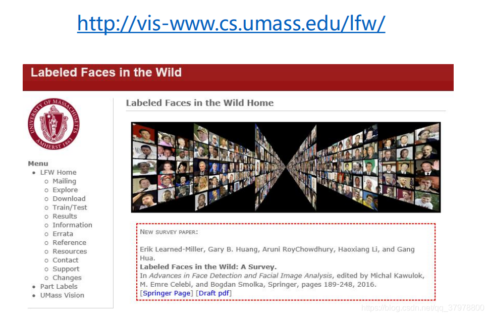
SVM-人脸识别

import matplotlib.pyplot as plt
from sklearn.model_selection import train_test_split
from sklearn.datasets import fetch_lfw_people
from sklearn.model_selection  import GridSearchCV
from sklearn.metrics import classification_report
from sklearn.svm import SVC
from sklearn.decomposition import PCA

# 载入数据

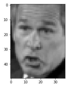
lfw_people = fetch_lfw_people(min_faces_per_person=70, resize=0.4)

plt.imshow(lfw_people.images[6],cmap='gray')
plt.show()

# 照片的数据格式
n_samples, h, w = lfw_people.images.shape
print(n_samples)
print(h)
print(w)

lfw_people.data.shape

lfw_people.target

target_names = lfw_people.target_names
target_names

n_classes = lfw_people.target_names.shape[0]

x_train, x_test, y_train, y_test = train_test_split(lfw_people.data, lfw_people.target)

model = SVC(kernel='rbf', class_weight='balanced')
model.fit(x_train, y_train)

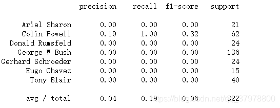
predictions = model.predict(x_test)
print(classification_report(y_test, predictions, target_names=lfw_people.target_names))

PCA降维

# 100个维度
n_components = 100

pca = PCA(n_components=n_components, whiten=True).fit(lfw_people.data)

x_train_pca = pca.transform(x_train)
x_test_pca = pca.transform(x_test)

x_train_pca.shape

model = SVC(kernel='rbf', class_weight='balanced')
model.fit(x_train_pca, y_train)

predictions = model.predict(x_test_pca)
print(classification_report(y_test, predictions, target_names=target_names))

调参

param_grid = {'C': [0.1, 1, 5, 10, 100],
              'gamma': [0.0005, 0.001, 0.005, 0.01], }
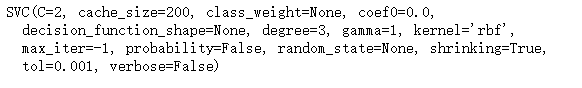
model = GridSearchCV(SVC(kernel='rbf', class_weight='balanced'), param_grid)
model.fit(x_train_pca, y_train)
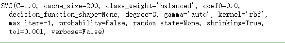
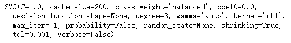
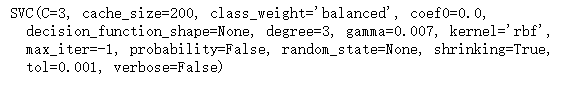
print(model.best_estimator_)

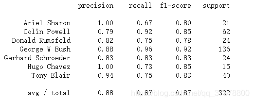
predictions = model.predict(x_test_pca)
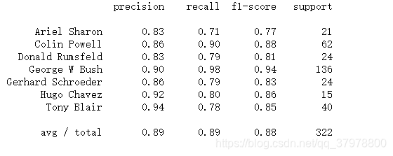
print(classification_report(y_test, predictions, target_names=target_names))

param_grid = {'C': [0.1, 0.6, 1, 2, 3],
              'gamma': [0.003, 0.004, 0.005, 0.006, 0.007], }
model = GridSearchCV(SVC(kernel='rbf', class_weight='balanced'), param_grid)
model.fit(x_train_pca, y_train)
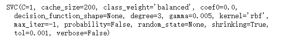
print(model.best_estimator_)

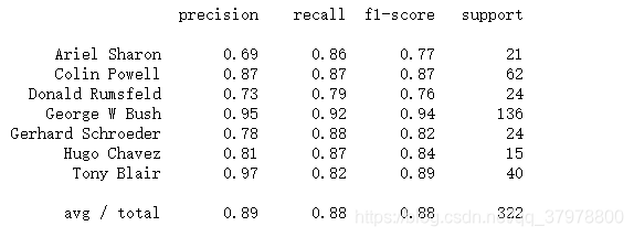
predictions = model.predict(x_test_pca)
print(classification_report(y_test, predictions, target_names=target_names))

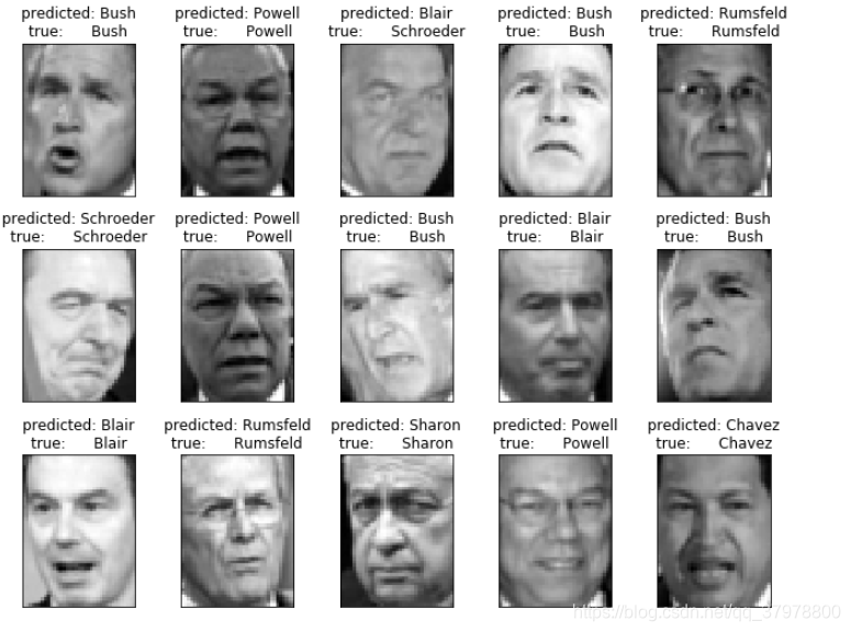
画图

# 画图，3行4列
def plot_gallery(images, titles, h, w, n_row=3, n_col=5):
    plt.figure(figsize=(1.8 * n_col, 2.4 * n_row))
    plt.subplots_adjust(bottom=0, left=.01, right=.99, top=.90, hspace=.35)
    for i in range(n_row * n_col):
        plt.subplot(n_row, n_col, i + 1)
        plt.imshow(images[i].reshape((h, w)), cmap=plt.cm.gray)
        plt.title(titles[i], size=12)
        plt.xticks(())
        plt.yticks(())

# 获取一张图片title
def title(predictions, y_test, target_names, i):
    pred_name = target_names[predictions[i]].split(' ')[-1]
    true_name = target_names[y_test[i]].split(' ')[-1]
    return 'predicted: %s\ntrue:      %s' % (pred_name, true_name)

# 获取所有图片title
prediction_titles = [title(predictions, y_test, target_names, i) for i in range(len(predictions))]

# 画图
plot_gallery(x_test, prediction_titles, h, w)

plt.show()