


1.参考文献
青藏高原的范围以青藏高原科学数据中心的TPBoundary_new (2021)矢量数据为准。
国家青藏高原科学数据中心![]() https://data.tpdc.ac.cn/zh-hans/data/61701a2b-31e5-41bf-b0a3-607c2a9bd3b3
https://data.tpdc.ac.cn/zh-hans/data/61701a2b-31e5-41bf-b0a3-607c2a9bd3b3
此处主要是对水要素进行变化检测,MK趋势分析方法主要参照这篇论文:
于延胜,陈兴伟.R/S和Mann-Kendall法综合分析水文时间序列未来的趋势特征[J].水资源与水工程学报,2008(03):41-44.
在下面这篇博客的基础上进行修改:
 https://blog.csdn.net/wlh2067/article/details/129712105?utm_medium=distribute.pc_relevant.none-task-blog-2~default~baidujs_baidulandingword~default-8-129712105-blog-112796872.235^v28^pc_relevant_recovery_v2&spm=1001.2101.3001.4242.5&utm_relevant_index=11
2.方法介绍
2.1MK趋势分析
Kendall法是一种被广泛用于分析趋势变化特征的检验方法,它不仅可以检验时间序列趋势上升与下降,而 且还可以说明趋势变化的程度,能很好地描述时间 序列的趋势特征。
1. 对于一个独立、随机同变量分布的时间数据序列(x1,x 2 ,…,xn),其正态分布的检验统计变量S为:

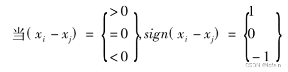
其中,i>j,即后减前。
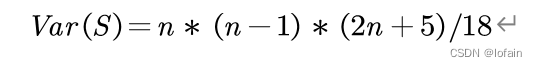
2.计算方差:
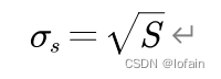
标准差:
3.计算检验值Z:
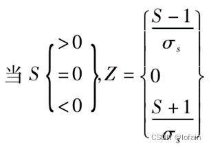
若Z>0,检验的时间序列为上升变化趋势,Z<0, 检验的时间序列为上下降变化趋势;Z的绝对值大 于或等于2.32、1.64、1.28,表示通过置信度分别为 99%、95%以及90%的显著性检验水平。
2.2Sen's slope计算趋势斜率
在Mann-Kendall检验确定存在趋势后,可以使用Sen's slope来计算趋势的斜率。Sen's slope是一种计算趋势斜率的方法,它利用中位数差来估计趋势的斜率,与线性回归方法不同,Sen's slope不受异常值的影响,因此更适用于含有异常值的数据。Sen's slope表示时间序列中单位时间的变化量。当Sen's slope为正数时,表示时间序列呈现上升趋势,当Sen's slope为负数时,表示时间序列呈现下降趋势。
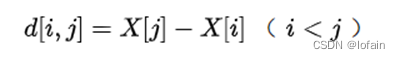
1.对于长度为n的时间序列X,计算n(n-1)/2个变量关系差(d):
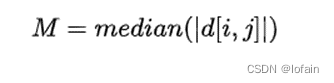
2.计算所有d[i,j]的绝对值的中位数:
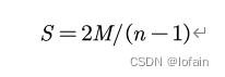
3.计算Sen's slope:
3.完整代码与改动介绍
var table = ee.FeatureCollection("users/20220404g/TPBoundary_new");
Map.centerObject(table,5);

//!bandName
var bandName="water";
//!dataset,time
var data=ee.ImageCollection("JRC/GSW1_4/MonthlyHistory")
            .filterDate('1990-01-01','2002-01-02')
            .select(bandName);
//print(testData)
//---------------------

var List=data.map(
  function(image){
    var date=ee.Date(image.get('system:time_start'));
    var date1= date.difference(ee.Date('2000-01-01'), 'year');
    var imageNew=image.addBands(ee.Image.constant(date1).toFloat()).clip(table);
    return imageNew;
});
var afterFilter = ee.Filter.lessThan({
  leftField: 'system:time_start',
  rightField: 'system:time_start'
});
var coll=List.select(bandName);
var join=ee.ImageCollection(ee.Join.saveAll('after').apply({
  primary: coll,
  secondary: coll,
  condition: afterFilter
}));
//Saves all images after the current image in a property of the current image
//print(snowJoin)
function sign(i,j){
  //i and j are images:
  var diff=j.subtract(i);
  return diff.gt(0).multiply(1).add(diff.eq(0).multiply(1)).add(diff.lt(0).multiply(-1));
}
var kendall=ee.ImageCollection(
  //kendall is a image
  join.map(
    function(current){
      var afterImageCollection=ee.ImageCollection.fromImages(current.get('after'));
      return afterImageCollection.map(
        function(image){
          return sign(current, image).unmask(0);
        });
    }
    ).flatten())
    .reduce('sum', 2)//2 is location
    .clip(table)
    .float();//!
//Calculate the difference between n(n-1)/2 variables
print("done:compute S");
//--------------------

var slope=function(i, j) { // i and j are images
  return ee.Image(j).subtract(i)
      .divide(ee.Image(j).date().difference(ee.Image(i).date(),'year'))
      .rename('slope')
      .float();
};
var slopes=ee.ImageCollection(join.map(function(current) {
  var afterCollection = ee.ImageCollection.fromImages(current.get('after'));
  return afterCollection.map(function(image) {
      return ee.Image(slope(current, image));
  });
}).flatten());
//print(slopes)
var sensSlope = slopes.reduce(ee.Reducer.median(), 2).float();
//Calculate the median of the absolute values of all d[i,j]
print("done:compute SensSlope")
//----------------

// Values that are in a group (ties).  Set all else to zero.
var groups = coll.map(function(i) {
  var matches = coll.map(function(j) {
    return i.eq(j); // i and j are images.
  }).sum();
  return i.multiply(matches.gt(1));
});

// Compute tie group sizes in a sequence.  The first group is discarded.
var group = function(array) {
  var length = array.arrayLength(0);
  // Array of indices.  These are 1-indexed.
  var indices = ee.Image([1])
      .arrayRepeat(0, length)
      .arrayAccum(0, ee.Reducer.sum())
      .toArray(1);
  var sorted = array.arraySort();
  var left = sorted.arraySlice(0, 1);
  var right = sorted.arraySlice(0, 0, -1);
  // Indices of the end of runs.
  var mask = left.neq(right)
  // Always keep the last index, the end of the sequence.
      .arrayCat(ee.Image(ee.Array([[1]])), 0);
  var runIndices = indices.arrayMask(mask);
  // Subtract the indices to get run lengths.
  var groupSizes = runIndices.arraySlice(0, 1)
      .subtract(runIndices.arraySlice(0, 0, -1));
  return groupSizes;
};

// See equation 2.6 in Sen (1968).
var factors = function(image) {
  return image.expression('b() * (b() - 1) * (b() * 2 + 5)');
};

var groupSizes = group(groups.toArray());
var groupFactors = factors(groupSizes);
var groupFactorSum = groupFactors.arrayReduce('sum', [0])
      .arrayGet([0, 0]);

var count = join.count();

var kendallVariance = factors(count)
    .subtract(groupFactorSum)
    .divide(18)
    .float();
print("done:kendallVariance")
//------------------


var trendVis = {
  palette:[
    '040274', '040281', '0502a3', '0502b8', '0502ce', '0502e6',
    '0602ff', '235cb1', '307ef3', '269db1', '30c8e2', '32d3ef',
    '3be285', '3ff38f', '86e26f', '3ae237', 'b5e22e', 'd6e21f',
    'fff705', 'ffd611', 'ffb613', 'ff8b13', 'ff6e08', 'ff500d',
    'ff0000', 'de0101', 'c21301', 'a71001', '911003'
  ],
  min:-10000,
  max:10000
};
//red mean up,blue mean down

//!export:kendall,sensSlope,kendallVariance,z
Export.image.toDrive({
  image:kendall,//!turn the name
  description: 'k_jcr_9002',//!turn the name too,You need to write in format
  scale: 30,//!Be determined by the data and be as clear as possible
  region:table,//
  maxPixels:1e13,
  fileFormat: 'GeoTIFF'
}
);
print("done:export data");


//Map.addLayer(List.select(bandName), trendVis,bandName);
Map.addLayer(kendall, trendVis, "kendall");
3.改动说明
数据集和一些显示设置的改动就不介绍了,主要介绍对算法的重大改动。
3.1sign函数
sign函数要求输入两个图像j和i,使用j图像减去i图像,对于每个像元,如果结果大于0则返回1,如果结果等于0则返回0,如果结果小于0则返回-1。
原博客sign函数,使用python编写:
def sign(i, j):  # i and j are images:
    return ee.Image(j).neq(i).multiply(ee.Image(j).subtract(i).clamp(-1, 1)).int()
改动后:
function sign(i,j){
  //i and j are images:
  var diff=j.subtract(i);
  return diff.gt(0).multiply(1).add(diff.eq(0).multiply(1)).add(diff.lt(0).multiply(-1));
}
如果使用ECMWF/ERA5_LAND/MONTHLY_AGGR其中的snow_depth_water_equivalent波段,某些地方像元值会非常的小,只有0.005左右:
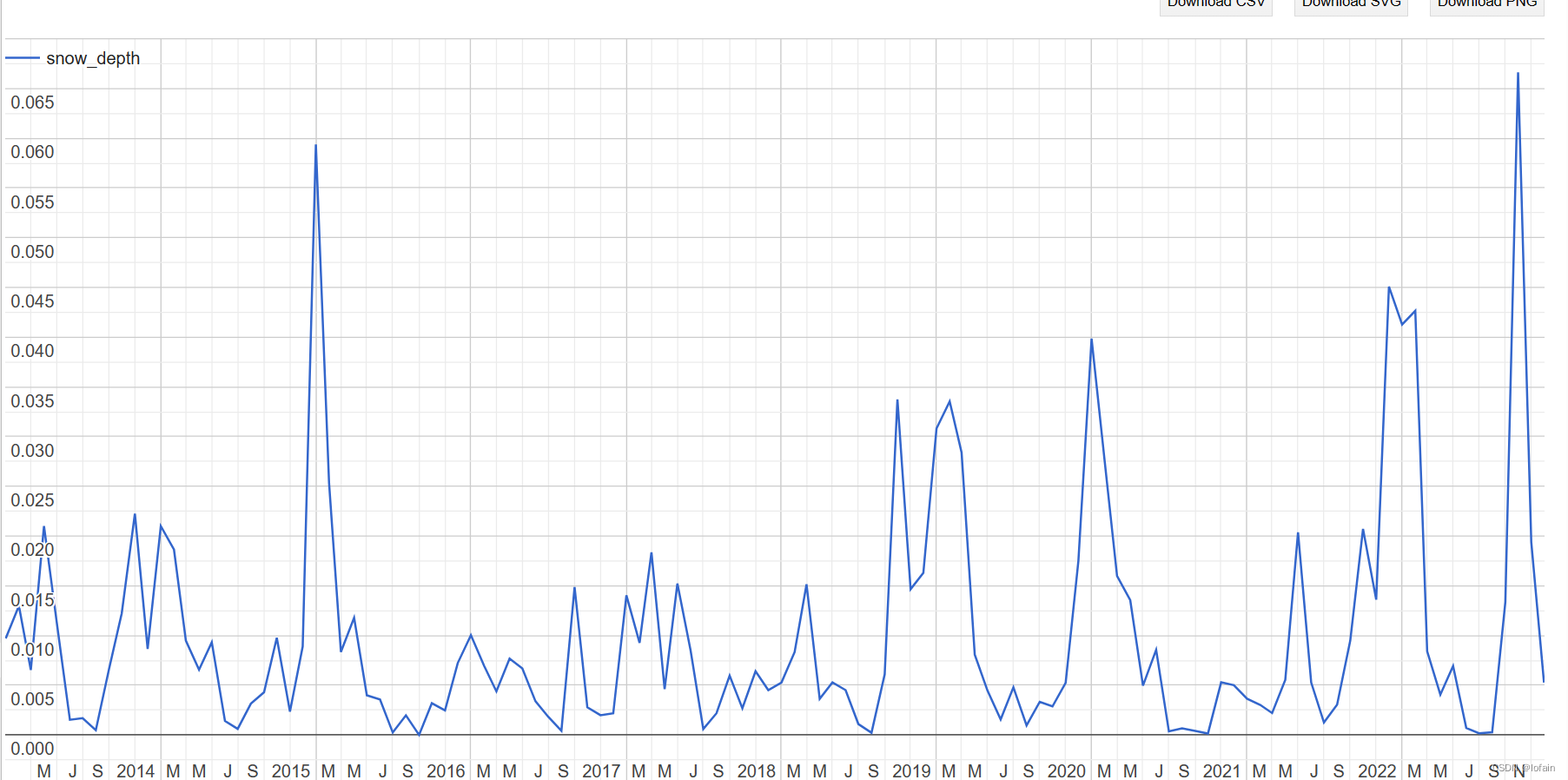
原函数先比较了下j和i的值,如果相同就直接为0。把j减i的值映射到-1到1之间转为乘给j,最后转为整数。我不太懂这里为什么要用乘,但是使用clamp,映射到(-1,1)会有一个问题,如果像元值太小,比如前一个值为0.005,后一个值为0.008,相减后得到0.003不会变为1而是直接转化为0。
如果像元值都比较大,比如几十上百这种,就不会有什么问题,但是绝对值远小于1的数据,会全部被转换为0,而得不到变化趋势。
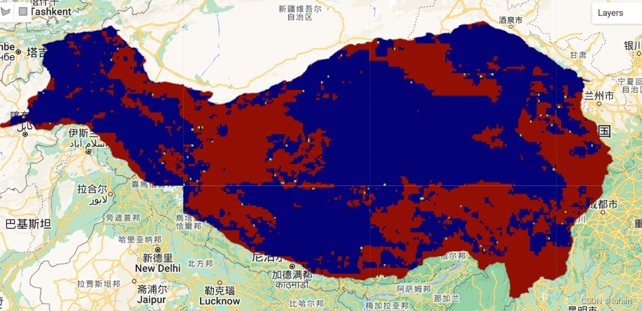
改进后的函数将两个图像的差值与0进行比较,就能够避免这种问题。选取ECMWF/ERA5_LAND/MONTHLY_AGGR的snow_depth_water_equivalent波段十年左右的数据,改进前后对比:
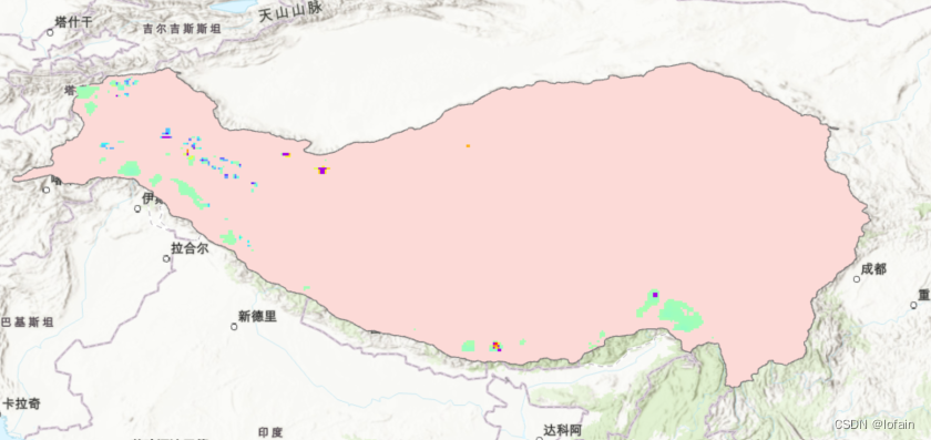
(没用像元的地方,值全部是0)
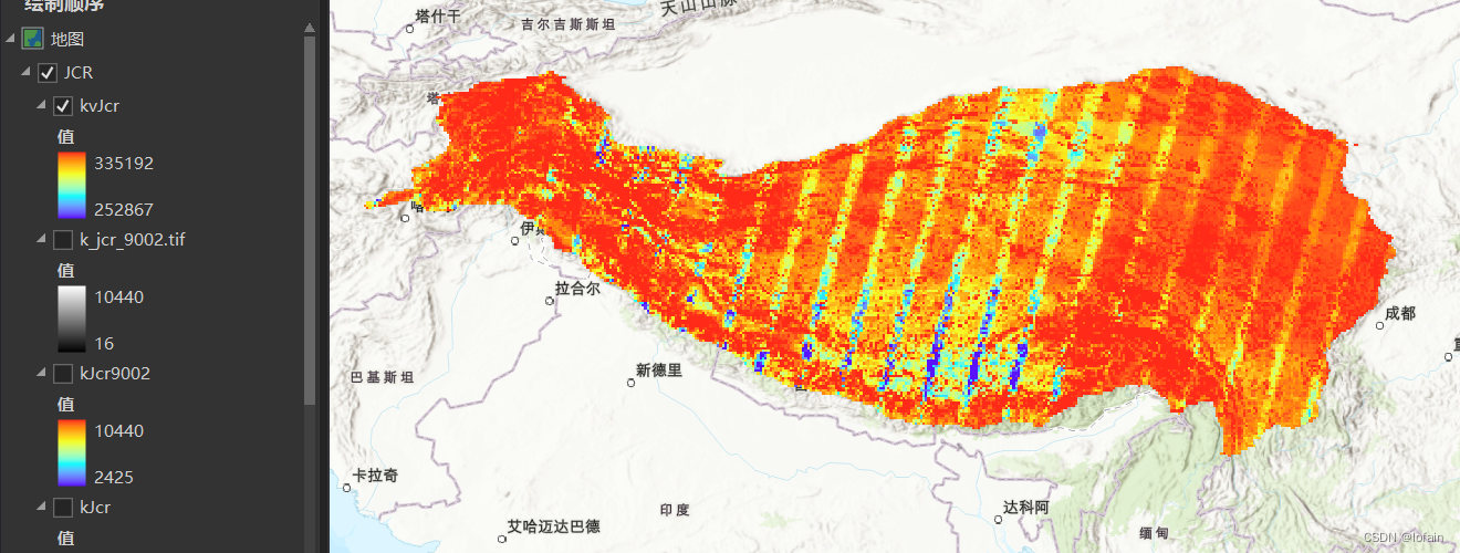
 4.计算结果
下面这些图像是最终可以得到的结果,此处以jcr做展示,由于是在不同代码版本下跑的,不是百分百正确,因此仅用于展示能得到哪些结果。
4.1检验统计变量S
S,代码里为kendall,能大概说明哪些地方发生改变以及变化的程度。
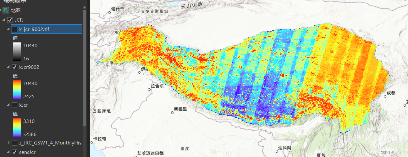
4.2斜率sensSlope
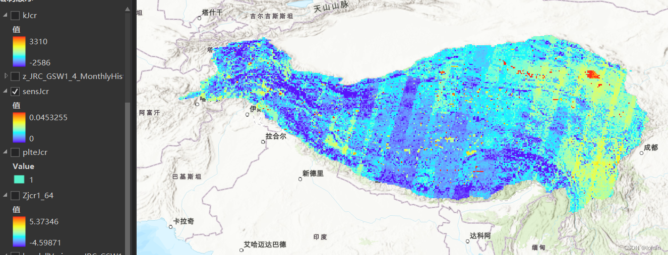
4.3 方差
4.4检验值Z
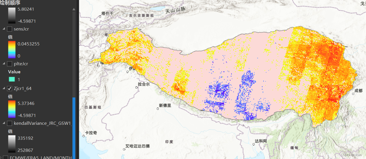
大于1.64或小于-1.64表明有95%的显著性检验水平。
FIN


 1732
1732

 被折叠的 条评论
为什么被折叠?
被折叠的 条评论
为什么被折叠?
 到【灌水乐园】发言


