SIGNED DISTANCE FIELD RENDERING JOURNEY PT.2

最新推荐文章于 2022-10-23 13:59:58 发布

未寒

最新推荐文章于 2022-10-23 13:59:58 发布

阅读量611

点赞数

Hi guys,

Disclaimer: This post is not an overview of signed distance fields, nor is it a guide on how to create them/work with them.
I will write a more comprehensive post about the whole topic in future once I’ve “finished” the implementation.

Note: Usually all my code is available on github, but as this is WIP I’m currently using a private local branch. You can try this stuff at a later date when it’s working and I have a basic scene setup again.

This is more or less a documentary of my “journey” to integrate SDF into my engine.

Alright, welcome back to the SDF journey :)

If you are not up to what I have done so far – here is part one again.

The main goal now was to expand our technique to work with multiple volume textures, both from multiple instances of the same signed distance field and different meshes altogether.
This weekend I didn’t have as much time, and so the results might not be as satisfactory, I apologize. Also note that I will focus more on other things (like learning OpenGL) in the coming weeks, so progress is halted.

So a lot of what is written here is more of an “outlook” on what I’ll do next instead of showing off awesome new stuff. Some awesome new stuff is in though!

SDF Generation revisited

In order to work with multiple meshes I first wanted to find a suitable, interesting mesh to add to my collection.

I came back to this guy you see on the right (the famous “Stanford dragon”, find here) which I usually use to test out new stuff.

The reason I abstained from that is that this model has over a million polygons alone, so I totally ruled it out for CPU SDF generation. I later went on to use Blender’s “decimate” feature to bring that down to a more reasonable amount (and learn how to bake normal maps along the way!).

However, it turns out that our SDF has some slight errors still. Because of how my ray marching visualizer works these manifest in lines of points.

In the last article I mentioned how I use ray tracing to check if we are inside a mesh (if from any given point we cast a ray, we can say we are “inside” if the number of mesh intersections is uneven) and how that solved my previous problems.

A new “problem” emerges – what if our mesh is not properly closed? It seems to be the case for the Stanford dragon, or at least my low-poly representation – the model (which originally is built from real-life 3d scan data – always a bit noisy) does exhibit small holes or overlaps and even a bunch of useless triangles inside the mesh.

My original code for determining whether we are inside or outside simply checked whether or not the closest triangle was back or front facing, but that didn’t work well. I then tried to apply a weight based on the inverse distance to every triangle as the determining factor (logic: If most “close” triangles are facing away we are inside!), but that went wrong, too. So I later came up with the ray casting idea.

I checked the Unreal paper (Dynamic Occlusion with SDFs) again, and they determine “inside” when >50% of the triangles hits are back faces. The upside of that algorithm is that it can work with meshes that are open at the bottom; for example a lot of environment props like lamps, houses etc. do not need these triangles since they are always sitting on top of some ground.

It’s easy, however, to come up with scenarios where this method would break – for example imagine a building with a highly detailed shop or façade on one side and only few quads to cover the other sides –> if we are behind (and outside!) the building most triangles are facing backwards towards the sample point, indicating a possible “being outside” of the sample point.

One could always give a range limit on what triangles should contribute to this heuristic, but hard limits are not useful (think different mesh sizes, or different sample resolutions) and I do not want the person who uses my tools to learn this part, too (myself included)

Or one could use occlusion, and discard the triangles that are not visible from the sample point. But this would be very, very expensive.

EDIT: Daniel Wright, the author of the Unreal solution, pointed out: “The rays being traced are first hit rays, so they would all hit the few quads in that case, giving the correct result (outside) for positions behind the building.”

So, I am sorry to say, I have not found the golden answer here, but I thought these things might be interesting should you look to implement SDF rendering into your engine.

It might also help to not use broken meshes in general. :)

Note: It’s something I didn’t notice immediately and also I did not have the skill to easily fix the dragon mesh, and I did not change my algorithm, so you will see some “spikes” sticking out of the dragon when looking at shadows etc. in the images below.

Multiple instances

I didn’t pursue answers to the SDF generation problem, but instead focused on expanding my previous work to be able to handle more than one object.

The first steps were pretty simple – we divide the information about the SDF into the actual texture information and the instance information.

So even though I only use one signed distance field, I have multiple instances with their specific transformations (translation and rotation in a matrix, scale separately, see here).

So then for our distance function we have to loop through all instances and use the minimum value as our result.

Our efficiency is obviously linearly tied to the amount of meshes then, which is not great at all. But let’s worry about that later.

Multiple different meshes

A much more interesting step then was to have multiple SDFs be represented in one scene.

It really helps that I store the SDFs as 2d textures, which, as a reminder, typically have the resolution of 2500 x 50 (so 50 samples in each direction), but the size can vary depending on requirements.
We really do not want to submit multiple textures to our pixel shader to choose from, and we do not want to deal with arrays, either. Both of these methods are very static and inflexible.

The solution I went with is to create a large texture (atlas) which contains all the SDF textures. I update this texture only when new SDFs are part of the scene, or if old ones are no longer used.

Usually filling up a texture atlas with differently sized small blocks is a really exciting problem, which I attempted to solve for an HTML game a while ago (see on the right).
I basically needed to precompute differently sized space ship sprites, but didn’t want to deal with hundreds of separate textures.

Anyways, just a small side note on these atlasses.

In our case we don’t really have to sort efficiently, since our SDFs are very very wide but not very tall, so it’s really more of a list and we arrange them one after another:

For each mesh instance we need to store

The mesh’s inverse transformation (translation, rotation, scale)
The mesh’s SDF index (in the array of SDFs)

For each SDF we need to store

the SDFs sample resolution (eg. 50x50x50)
the SDFs original scale, or, in other words, the distance between sampling points when the mesh is untransformed
the SDFs position in the texture atlas (in our case just the y-offset)

We then pass these arrays of instance information and SDF information to our shaders.

So that makes finding our minimum distance look like this:
For each instance:

Transform the current sample position/rotation to the instance position/rotation by multiplying with the inverse world matrix. Apply scale factor.
Get SDF information from the index stored in the instance
Sample this SDF
Compare to the previous minimum distance, and overwrite minimum if lower.

In code it looks like this (unfortunately this wordpress preset is not great for showing code)

for (uint i = 0; i < InstancesCount; i++)
{
float3 q = mul(float4(ro, 1), InstanceInverseMatrix[i]).xyz;

float dist = GetMinDistance(q / InstanceScale[i], InstanceSDFIndex[i]) * min(InstanceScale[i].x, min(InstanceScale[i].y, InstanceScale[i].z));

if (dist < minimum) minimum = dist;
}

It’s quite obvious that we do not want to check *every* SDF for every distance test, so in future I will try to optimize this process.

Calculating distance, revisited

Ok that’s something I previewed on the last blog post, but here I go again.

We assume that all our SDF sample points are accurate and give the correct minimum distance to any given geometry inside our volume.

I visualize this with a red sample point and a black circle/sphere which represents the mesh. The SDF’s bounding box is shown as the black outline around the volume.

However, a problem arises when we sample outside the SDF, since it’s essentially a black box from an outside perspective

So the naïve approach is to simply measure the shortest distance to the sdf volume and then add the sample distance at that point.

(distance inside the volume, distance toward the volume)

(both distances added)

The problem is evident – our “minimum” distance to the mesh is not correct – in fact – it is much too large. In the image below you can clearly see that

$∥ a∥ + ∥b ∥ >= ∥a + b ∥ = ∥c ∥ (which is also known as the triangle inequality)$

This is obviously a problem, since we can overshoot with our ray marching then! (Remember we always march with a step size equal to the minimum distance to any mesh, so that we can be sure to not hit anything during that step)

It should be noted that the error is usually not as large, since the SDF volume should align with the mesh’s bounding box. But there are many cases where this can be the case, think for example a chimney at the end of a house, or a car antenna. A vertical slice of the SDF would look similar to my drawing.

So how do we go about that?

Store more data

The problem is that we only store distance in our SDF, not direction. A good approximation of c would be to simply add a + b (as seen in the drawing above), so if we store the whole vector for each sample we are good to go.

A vector field still gives correct values when using linear interpolation, so it should work more or less right from the get-go.

The obvious issue is that we have to store at least 3 values now. If we choose float or half as our channel format we need to bump that to 4 (since that format only supports 1,2 and 4 channels).

This quadruples our memory and bandwidth requirements.

Gradient

The first idea I had was to simply test one more sample, which is located a “bit more” inside of the volume. Like so:

We calculate the gradient between the two sample points, and make a linear function to extrapolate to our original query point outside.

This changes basically nothing and is not a good idea, since distances obviously do not work like that. I made a quick graph to show how the real distance behaves.

The sample position for this graph is [1, y], and the distance is measured towards the origin. Our variable is the y value, so that would be the direction of the gradient.

[note to self: maybe make a drawing of that]

http://thetamath.com/app/y=sqrt((1+x%5E(2)))

The error obviously gets smaller and smaller once our distance becomes very large, and looks almost like a linear (absolute) function at some point. At that point the small x offset at the beginning is not important any more.

So, great, that might work for very large values, but at that point our original naïve implementation works well enough, too.

Sphere-sphere intersection

What I really want to know is the orientation of our distance vector inside the SDF, as explained earlier.

Here is a possible solution I came up with.

First of all – we know that our minimum distance basically describes a sphere (or circle in 2d) in which we can assume we hit nothing.

The basic idea then is to, again, sample another point which is pushed in a little in the direction of a (shortest-distance-to-volume vector) – this is the orange point in the gif below.

We can then assume both the red and orange sample points have distances which can represent spheres in which we hit nothing.

In 2d case, these are the red and orange circle.

With some simple math (“sphere sphere intersection”) we can calculate the points where these 2 meet. In case of 2d these are 1 or 2 points, in case of 3d we get a circle, basically what we get when we rotate the 2d points around our axis (line between red and orange).

The best visualization I have found is in this great answer at stackexchange. Check it out if you are interested in the math and results.

Anyways, what we have is the vector we wanted (intersection point – sample point one). We simply have to add it to the original vector a (closest point on the volume – outside sample point) and calculate its length to get the smallest distance.

Some of you may ask – but what about the second intersection point on the other side?
Well that’s the beauty of this method. It doesn’t matter. Since orange is displaced based on our incoming vector the other direction also yields the same distance in the end (check out the blue lines in the gif above!)

It’s also imperative that our second inside sample is very close to the first one, it absolutely should have a close point on the mesh represented.
That’s why it’s a good idea to leave some boundary with empty space when constructing the SDF.

Results?

Sadly, I didn’t have time to implement it into my engine, yet. I probably won’t have any time for SDFs in the coming days, but I wanted to write a little bit about my research. Hopefully part 3 will be more interesting, sorry again. Please don’t lynch me.

So it’s not clear whether that idea even works with real sdf data.

I did, however, implement a simple 2d shader on shadertoy that works with this idea for testing (Click on the image for a link!)

EDIT: David Farrell on twitter spun the gradient idea a bit further and came up with this scheme

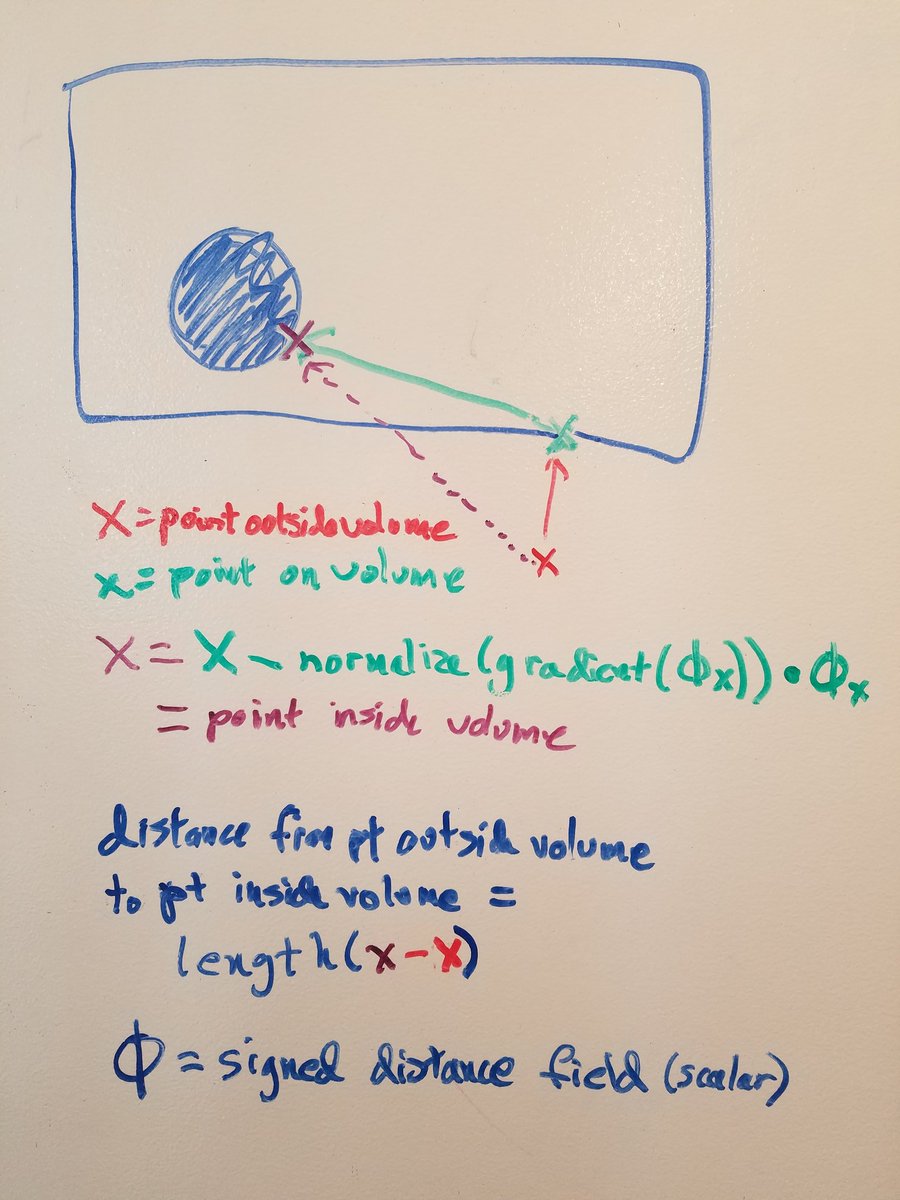
It makes perfect sense – we calculate the gradient at the border point which gives us the direction towards the closest mesh. If we normalize this vector and multiply it by the distance to the mesh our vector should end right at the mesh, which is what we want. Then we can just calculate the distance from our outside sample to this meshpoint and we have our resulting shortest distance.

The upside of this technique is the obvious simplicity. My shadertoy code looks like this

//x outside volume = fragCoord –> red
//x on volume = sampleBorder –> green

float phi = sdFunc(sampleBorder);
float d = 1.;
float grad_x = sdFunc(sampleBorder + vec2(d, 0)) – phi;
float grad_y = sdFunc(sampleBorder + vec2(0, d)) – phi; //in OpenGL positive Y points upwards

vec2 grad = vec2(grad_x, grad_y);

vec2 endpoint = sampleBorder – normalize(grad) * phi; // –> violet

sd = distance(endpoint, fragCoord);

If we sample 2 position (+d, 0 and 0, +d) for the gradient this technique has a higher texture read cost than the circle solution.

I quickly threw it into shadertoy, you can check it out side by side against circle intersection

Subsurface scattering

SDFs are both fairly accurate for small objects and can be used without regard for screen space limitations.

I thought – why not use it for subsurface scattering then?

The implementation took maybe 10 or 20 minutes and here are some results.

Since it was more of a quick idea I didn’t bother to look into physically plausible scattering or light absorption behavior for different materials.

Instead I just measured the distance the light travelled from entering the body to getting out again and then added a diffuse light term based on that.

Because SDFs work in world space this works out of the box without any big issues.

At first (in the gifs above) I thought I was being smart by ray marching from light towards the object and then calculate the SSS by the distance of the hitpoint to the pixel’s position. I figured it would be cheaper than going the other way because the light can skip a lot of space and only needs a few steps until it hits the object. If we start at the pixel’s position and move towards the light until we are “out” of the mesh we start out with very small distances and ray steps.

I obviously overlooked that the light might as well hit a different mesh altogether, which would result in wrong calculations!

So I corrected my ways when I went on to add shadows to our subsurface scattering.

Not only do we now travel from pixel position inside through the mesh until we are out – but we also continue our travel all the way to the light to see if we are in shadow.

We can also adjust the shadowing to be softer than our default shadowing, since subsurface scattering is usually very diffuse. You can see this in the image above. The shadow on the figure is pretty sharp on the front surface, but more diffuse on the back.

Note: Ideally we interpolate the shadow softness based on the distance the light travelled through the mesh

There are a bunch of problems with this approach that I would like to tackle in future iterations – the biggest one seems to be self-shadowing.

The issue is that if the light travels a short distance through the mesh, leaves the mesh, and then reenters the mesh again the second part will be treated as if it is in full shadow. This is not correct, since the light didn’t lose all power when traveling through the first part of the mesh ( remember – our mesh does not absorb all light with these sorts of materials!)

The universal answer to that would probably be to accumulate shadow darkness / light transmittance based on the materials it had to travel through.

Ambient Occlusion

Here is a total over-the-top image of the effect.

The basic idea is to travel in “each direction” of a hemisphere and check if we hit the sky. If so then add the sky color (or our environment cubemap’s color at that point) to our lighting term.

Obviously we cannot actually check each direction (there is no such thing, we could integrate over areas of our hemisphere), but we can use some easy tricks to “fake” or approximate some of that by ray marching in a direction and expanding our reference distance each time, which we compare to the SD at each sample.

The Unreal Engine 4 paper mentioned before is a really great resource for all of that

Regardless, this is just another sneak peek at what’s to come in the next part of this series!

Final words

I will leave it at that, since a proper explanation and implementation of some of these things take a bit of time and are more than enough to fill another post.

I do apologize to leave you guys hanging with a lot of unfinished things, but I prefer to write about stuff that is still “fresh in memory” as I will not have time in the near future to continue working on this project a lot.

Regardless, I hope you enjoyed the little content that was there :)

I’d be very glad if you have suggestions on what I can