机器学习：一元线性回归（梯度下降法）

目录

一、理论知识

1、一元线性回归模型（映射函数）

2、损失函数（代价函数）

3、梯度计算

4、梯度下降

二、代码实现

1、导入Python包

2、利用sklearn构造线性回归数据集

3、定义并初始化权重参数 W 和 b

4、前向传播函数：计算映射函数

5、损失计算函数

6、反向传播函数：梯度下降

7、数据预处理：特征归一化 + 调整维度

8、划分训练集和测试集

9、模型训练

10、模型测试

---

一、理论知识

1、一元线性回归模型（映射函数）

其中，表示输入，表示输出，和表示可学习的权重参数。

2、损失函数（代价函数）

其中，是标签，是预测值。

3、梯度计算

注：梯度计算遵循的是矩阵求导法则和链式求导法则。

4、梯度下降

其中，A是梯度下降步长，又称学习率。多次迭代执行前向传播（计算映射函数）和反向传播（梯度计算+梯度下降），损失函数最终收敛至局部最优解。

二、代码实现

1、导入Python包

import numpy as np
import matplotlib.pyplot as plt
from sklearn.model_selection import train_test_split
from sklearn.metrics import mean_squared_error
from sklearn.datasets import make_regression

plt.rcParams['font.sans-serif'] = ['Times New Roman']

2、利用sklearn构造线性回归数据集

X, Y = make_regression(n_samples=100, n_features=1, noise=50, random_state=2024)

plt.figure(dpi=100)
plt.scatter(X, Y)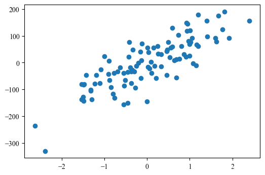

3、定义并初始化权重参数 W 和 b

weights = np.zeros((1, 1))
bias = 0

4、前向传播函数：计算映射函数

def forward(X, weights, bias):
    Y_hat = np.dot(X, weights) + bias
    return Y_hat

5、损失计算函数

def Loss_fuction(Y, Y_hat):
    N = Y.shape[0]
    cost = 1 / (2 * N) * np.sum((Y_hat - Y) ** 2)
    return cost

6、反向传播函数：梯度下降

def backward(X, Y, Y_hat, weights, bias, lr):
    # 梯度计算
    N = Y.shape[0]
    dw = 1 / N * np.dot(X.T, (Y_hat - Y))
    db = 1 / N * np.sum(Y_hat - Y)

    # 权重更新
    weights -= lr * dw
    bias -= lr * db
    return weights, bias

7、数据预处理：特征归一化 + 调整维度

X = (X - np.mean(X, axis=0, keepdims=True)) / (np.std(X, axis=0, keepdims=True) + 1e-8)
Y = Y[:, None]

8、划分训练集和测试集

X_train, X_test, Y_train, Y_test = train_test_split(X, Y, test_size=0.2, random_state=2024)
print(X_train.shape, X_test.shape, Y_train.shape, Y_test.shape)

(80, 1) (20, 1) (80, 1) (20, 1)

9、模型训练

lr = 0.01 # 学习率
epochs = 1000  # 迭代次数
train_loss = []
for _ in range(epochs):
    # 前向传播
    Y_hat = forward(X_train, weights, bias)

    # 损失计算
    loss = Loss_fuction(Y_train, Y_hat)
    train_loss.append(loss)

    # 反向传播
    weights, bias = backward(X_train, Y_train, Y_hat, weights, bias, lr)

plt.figure(dpi=100)
plt.plot(train_loss)
plt.xlabel("Epoch")
plt.ylabel("Loss")
plt.title("Training Loss")
plt.show()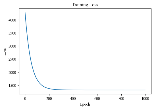

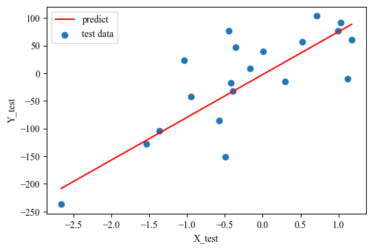
10、模型测试

plt.figure(dpi=100)
plt.scatter(X_test[:,0], Y_test[:,0], label='test data')
lin_x = np.linspace(np.min(X_test[:,0]), np.max(X_test[:,0]), 100)
lin_y = forward(lin_x[:,None], weights, bias)[:,0]
plt.plot(lin_x, lin_y, 'r', label='predict')
plt.legend()
plt.xlabel('X_test')
plt.ylabel('Y_test')
plt.show()

y_predict = forward(X_test, weights, bias)
print(f"Test MSE: {mean_squared_error(y_predict, Y_test)}")

Test MSE: 3130.9712952593727