2 State Estimation and Localization for Self-Driving Cars

前言：这真的是很难得全方位介绍自动驾驶的组成到实现（理论上），专注于无人驾驶方向的课程算是头一个了（其他课程好像花钱的挺贵，Coursera真心算是为想自学的人提供了一个便捷的方法——可以通过15天的申请申请全部课程）
我建议大家还是申请官方的课程编程作业和自动驾驶仿真真的很有必要入一下，做一下，才能理解一些模型的建立过程，代码的实现吧。

1. Coursera官方链接
2. b站搬运不是很高清的 CC英文字幕 但是UP主有建github 下载了视频和课件可以去看看评论区获取吧。
   尽管这样，我还是想强调一遍直接在Coursera申请助学金来听课是效果最好的，一来能督促自己（因为申请的课程是必须要通过的 不通过下次就不能申请其他课程了），二来编程作业只能通过会员/申请/付费来解锁。

希望这以下笔记，和解题答案思路等能给大家领个头，也一起共同学习进步，毕竟国内似乎还没有专门这么针对无人驾驶的课程专项。（为多伦多大学打call）

WEEK 1

Lesson 1: Practice Quiz

1.In order to apply the method of least squares, it is necessary to know the measurement noise variances.
False

2.For the method of least squares, select any/all that apply.
The method was pioneered by Carl Friedrich Gauss.
Given a linear observation model, the parameters that minimize the squared error criterion can be found by solving the normal equations.

3.According to the weighted squared error criterion, the error term corresponding to a measurement with a noise variance of 10 units will be weighted more highly than that of a measurement with a noise variance of 1 unit.
False

4.In which of these cases would the method of weighted least squares produce valid solutions. Select any/all that apply.
Ten measurements, two unknown parameters
Five measurements, five unknown parameters, and two different moise variances.
解释：Weighted least squares requires non-zero variances! Review the “Squared Error Criterion and the Method of Least Squares” lecture in this module.

5.You are measuring the voltage drop $V$ across an electrical component using two different multimeters; one of the meters is known to be more reliable than the other. Which method would you use to estimate the best voltage value from noisy measurements?
Weighted Least Squares

Lesson 2: Practice Quiz

1.The method of maximum likelihood gives the same parameter estimates as the method of least squares for any measurement noise distribution.
False

2.The product of several Gaussian PDFs with identical variances is also Gaussian.
True

3.The least squares criterion is robust to outliers.
False

4.For a scalar Gaussian random variable, what is the form of the full log likelihood function?
$-1/2log({\sigma }^2)$

5.True or False
False

Module 1: Graded Quiz

1.Measurements are drawn from a Gaussian distribution with variance ${\sigma }^2$. Which of the estimators below will provide the ‘best’ estimate of the true value of a parameter? Select any/all that apply:
Least Squares
Maximum Likelihood
Weighed Least Squares

2.Which of the following statements are correct? Select any/all that apply:
Least squares estimators are significantly affected by outliers.
When measurement noise comes from a large number of independent sources, a least squares estimator can be used.

3.Given the above histogram of noisy measurements, it is appropriate to use a LS estimator?
False

4.Looking at the histogram in the previous question, what could be the reason for such a distribution of measurements? Select any/all that apply:
The measured value might be changing.
There is an outside disturbance affecting the sensor.

WEEK 2

Module 3: Graded Quiz

1.Which of these statements are true? Select any/all that apply:
Every set of Euler angles corresponds to a unit quaternion.
Every unit quaternion has an associated 3x3 rotation matrix.

2.Which of these are valid rotation matrices? Select any/all that apply:
1 0 0;0 1 0;0 0 1
1 0 0;0 x x;0 -x x

3.Localization can be performed on board a vehicle by integrating the rotational velocities and linear accelerations measured by an IMU. Assuming that the IMU measurement noise is drawn from a normal distribution, what will the pose estimation error look like?
The vehicle pose estimation error will grow with time.

4.Each GPS satellite transmits a signal that encodes:
The satellite’s position and time of signal transmission

5.Which of these systems provides the most accurate positioning measurement?
RTK GPS

6.What is the minimum number of GPS satellites required to estimate the 3D position of a vehicle through trilateration?
4

Module 4: Graded Quiz

1.A single 3D LIDAR reading consists of elevation, azimuth and range measurements
(3.9242, 0.6946, 0.3433)

2.A 3D LIDAR unit is scanning a surface that is approximately planar, returning range, elevation and azimuth measurements. In order to estimate the equation of the surface in parametric form (as a plane), we need to find a set of parameters that best fit the measurements.

Implement the sph_to_cat and estimate_params functions, which transform LIDAR measurements into a Cartesian coordinate frame and estimate the plane parameters, respectively. You may assume that measurement noise is negligible. The code comments provide more information on the format of the arguments to each function.

from numpy import *
from numpy.linalg import inv

def sph_to_cart(epsilon, alpha, r):
  """
  Transform sensor readings to Cartesian coordinates in the sensor
  frame. The values of epsilon and alpha are given in radians, while 
  r is in metres. Epsilon is the elevation angle and alpha is the
  azimuth angle (i.e., in the x,y plane).
  """
  p = zeros(3)  # Position vector 
  
  # Your code here
  p[0]=r*cos(alpha)*cos(epsilon)
  p[1]=r*sin(alpha)*cos(epsilon)
  p[2]=r*sin(epsilon)
  return p
  
def estimate_params(P):
  """
  Estimate parameters from sensor readings in the Cartesian frame.
  Each row in the P matrix contains a single 3D point measurement;
  the matrix P has size n x 3 (for n points). The format is:
  
  P = [[x1, y1, z1],
       [x2, x2, z2], ...]
       
  where all coordinate values are in metres. Three parameters are
  required to fit the plane, a, b, and c, according to the equation
  
  z = a + bx + cy
  
  The function should retrn the parameters as a NumPy array of size
  three, in the order [a, b, c].
  """
  param_est = zeros(3)
  
  # Your code here
  A = ones_like(P)
  b = zeros((P.shape[0], 1))

  for i, meas in enumerate(P):
    A[i, 1], A[i, 2], b[i] = meas
  
  param=inv(A.T@A)@A.T@b
  
  param_est[0]=param[0,0]
  param_est[1]=param[1,0]
  param_est[2]=param[2,0]
  
  return param_est
  
meas = array([[pi/3, 0, 5],
                 [pi/4, pi/4, 7],
                 [pi/6, pi/2, 4],
                 [pi/5, 3*pi/4, 6],
                 [pi/8, pi, 3]])
P = array([sph_to_cart(*row) for row in meas])
print(estimate_params(P))

3.Which of the following statements are true? Select any/all that apply.
ICP is sensitive to outliers caused by moving objects.
解释：Beacuse选项：Incorrect! While the points themselves lie in Euclidean space, the transformation between point clouds is defined by a translation and a 3D rotation. Rotations belong to the group called SO(3) and require special treatment. You can find more details on ICP in the “Pose Estimation from LIDAR Data” lesson of this module.

4.You are testing an algorithm for LIDAR-based localization on a vehicle in a controlled environment. What are some of the things you need to take into account? Select any/all that apply.
When the vehicle is moving quickly, it is important to account for the time differences between individual LIDAR pulses.
It is important to identify shiny and highly reflective objects in the environment, as LIDAR measurements of those objects may be invalid.

5.To estimate the motion of a self-driving car, it is necessary to transform LIDAR scan points from the sensor frame to the vehicle frame. The rotation of the vehicle frame with respect to the LIDAR frame is represented by the rotation matrix
Cp

WEEK 5

Final Project: Vehicle State Estimation on a Roadway

先统一贴一些问题（讨论区和我自己不太理解的地方） 有些是英文，大家还是习惯习惯吧，毕竟课程也是英文的嘛，能看到这里的估计都能看懂的：

1. In order to update the position estimate p_est[k], I need to multiply the C_{ns} with the f_{k-1} and then add gravity. I understand how gravity and the force from IMU is given in the code but I can not understand what’s up with C_{ns}.
   Can somebody help me understand how to express C_{ns} in the code?
2. In order to update the orientation estimate, I think I need to use the Quaternion.quat_mult(self, q) method given in the rotations.py script.
   Ok, I have the p_est[k-1] and the delta_t, as well as imu_w.data[k-1].
   What’s up with the ‘Ω’ and the ‘q’ in the beginning of it? I think ‘Ω’ has to do with Quaternion but I do not know what’s up with the ‘q’.
3. I cannot seem to figure out how q(omega * delta_t), q(theta) and big_omega(q) work out. if the u vector is 6 elements, then little omega is a vector with 3 elements: separate angular rates for x, y and z axes. If that is true, then little_omega * delta_t should produce a vector with 3 angles for the x, y and z axes. The definition shown in the slides makes it unclear how theta (a single angle) is derived from little_omega * delta_t (a vector) and how q(theta) turns into the quaternion passed to big_omega.
   In the axis-angle interpretation of quaternions, there is a single angle theta associated with an axis A = (x_0, y_0, z_0). A quaternion, a + bi + cj + dk, is defined from the axis-angle vales as: a = cos(theta/2), b = x_0 * sin(theta/2), c = y_0 * sin(theta/2), and d = z_0 * sin(theta/2). It’s not clear how this definition is implemented with the definitions shown in the slides.

所有的以上问题，其实在视频课件中有讲解（就是有些很浅，得看补充材料和相关论文），贴一下比较重要和代码也很相关的图（Motion Model十分重要 这也是验证代码非常重要的一个步骤）：

接下来可以回答问题了：（此回答参考：指向课堂讨论区）

1. Cns is the rotation matrix associated with quaternion qk-1
2. Ω is the term sigma in the function quat_mult in rotations.py which can be used to multiply two quaternions
3. You are right about then little_omega * delta_t should produce a vector with 3 angles for the x, y and z axes. And here Big_omega(little_omega * delta_t) means that we exchange it to Quaternion As we all know that q_est/q is # orientation estimates as quaternions. then it corresponding quat_mult_right which is Quaternion multiplication operation - in this case, perform multiplication on the right, that is, q*self. (More detail see in rotations.py)
   and it just corresponding to the third equation as the picture shown front.

好了那么开始代码部分的解释了，首先这个题挺难的，一是虽然课程组包装好了rotations.py但是！你是要看的不然根本不会用（这一点不像深度学习那边，凡是陌生函数都给使用方法和示例），不过这样一来也更能理解模型（真的很能）
这里我一个个解释，如果想看整体的请直接拖到最后（会放整个.py文件怎么写的）
1 是根据IMU进行的状态更新就和上一幅图的公式一一对应，就连Ω的问题我当时也有，在讨论区看了一会 自己想了一会就写了那个英文答案，大概就是内部的小q是四元数的形式（所以角速度成为需要转换的），大Ω是一种运算需要用到quat_mult_right，不过用之前必须先经过Quaternion的转换

    # 1. Update state with IMU inputs
    C_ns=Quaternion(*q_est[k-1]).to_mat()
    
    p_est[k]=p_est[k-1]+delta_t*v_est[k-1]+delta_t**2/2*(C_ns @ imu_f.data[k - 1] + g) #position
    v_est[k]=v_est[k-1]+delta_t*(C_ns @ imu_f.data[k - 1] + g)
    q_est[k]=Quaternion(axis_angle=imu_w.data[k-1]*delta_t).quat_mult_right(q_est[k-1])
   

2 emm 这个比较容易看懂了直接上ppt里的截图了

然后就是整个位置的不确定性通过线性模型的更新了：（我觉得我写的很详细了 希望大家都能看懂吧… 后面再贴一个我的笔记截图（图个++解释… 虽然写的不太好））

    # 1.1 Linearize the motion model and compute Jacobians
    F[0:3,3:6]=np.eye(3)*delta_t
    F[3:6,6:]=skew_symmetric(C_ns @ imu_f.data[k - 1])*delta_t
    
    Q[:3,:3]=var_imu_f*delta_t**2*np.eye(3)
    Q[3:,3:,]=var_imu_w*delta_t**2*np.eye(3)
    
    # 2. Propagate uncertainty
    p_cov[k] = F @ p_cov[k-1] @ F.T + l_jac @ Q @ l_jac.T #F @ p_cov or F @ p_est 均可

好了接下来就是ES_EKF怎么用来融合三个传感器进行更新的操作了（注意时间戳是不一样的，也就是说传感器的传送数据的频率是不同的，可能IMU的数据有了 GPS还没有，LIDAR还慢点，所以需要三者都有才更新 -> 没错 if一下）
emmm 我突然担心万一我毕设查重又查到这个博客了，emm 所以我少写点字多点截图笔记好了… hhhh

    # 3. Check availability of GNSS and LIDAR measurements
    # if条件两个:1 不超过最大的时间戳；2和现在k-1时刻imu的时间戳相同，因为是预测预估所以是k-1而不是k
    if lidar_i<lidar.t.shape[0] and lidar.t[lidar_i]==imu_f.t[k-1]:
        p_est[k], v_est[k], q_est[k], p_cov[k] = measurement_update(var_lidar, p_cov[k], lidar.data[lidar_i].T, p_est[k], v_est[k], q_est[k])
        lidar_i += 1 #1次过后 进入等待下一个lidar.t的时间
    # gnss也就是GPS是一个if道理
    if gnss_i<lidar.t.shape[0] and gnss.t[gnss_i]==imu_f.t[k-1]: 
        p_est[k], v_est[k], q_est[k], p_cov[k] = measurement_update(var_gnss, p_cov[k], gnss.data[gnss_i].T, p_est[k], v_est[k], q_est[k])
        gnss_i += 1

最后！重头戏啦，就是三者融合的更新函数的写法了：

# Main code for the Coursera SDC Course 2 final project
#
# Author: Trevor Ablett
# University of Toronto Institute for Aerospace Studies

from math import cos, sin
import pickle
import sys
import numpy as np
from numpy.linalg import norm, inv
import matplotlib.pyplot as plt
from mpl_toolkits.mplot3d import Axes3D

from rotations import Quaternion, skew_symmetric
sys.path.append('./data')

#### 1. Data ###################################################################################

################################################################################################
# This is where you will load the data from the pickle files. For parts 1 and 2, you will use
# p1_data.pkl. For part 3, you will use p3_data.pkl.
################################################################################################
with open('data/p1_data.pkl', 'rb') as file:
    data = pickle.load(file)

################################################################################################
# Each element of the data dictionary is stored as an item from the data dictionary, which we
# will store in local variables, described by the following:
#   gt: Data object containing ground truth. with the following fields:
#     a: Acceleration of the vehicle, in the inertial frame
#     v: Velocity of the vehicle, in the inertial frame
#     p: Position of the vehicle, in the inertial frame
#     alpha: Rotational acceleration of the vehicle, in the inertial frame
#     w: Rotational velocity of the vehicle, in the inertial frame
#     r: Rotational position of the vehicle, in Euler (XYZ) angles in the inertial frame
#     _t: Timestamp in ms.
#   imu_f: StampedData object with the imu specific force data (given in vehicle frame).
#     data: The actual data
#     t: Timestamps in ms.
#   imu_w: StampedData object with the imu rotational velocity (given in the vehicle frame).
#     data: The actual data
#     t: Timestamps in ms.
#   gnss: StampedData object with the GNSS data.
#     data: The actual data
#     t: Timestamps in ms.
#   lidar: StampedData object with the LIDAR data (positions only).
#     data: The actual data
#     t: Timestamps in ms.
################################################################################################
gt = data['gt']
imu_f = data['imu_f']
imu_w = data['imu_w']
gnss = data['gnss']
lidar = data['lidar']

################################################################################################
# Let's plot the ground truth trajectory to see what it looks like. When you're testing your
# code later, feel free to comment this out.
################################################################################################
'''
gt_fig = plt.figure()
ax = gt_fig.add_subplot(111, projection='3d')
ax.plot(gt.p[:,0], gt.p[:,1], gt.p[:,2])
ax.set_xlabel('x [m]')
ax.set_ylabel('y [m]')
ax.set_zlabel('z [m]')
ax.set_title('Ground Truth trajectory')
ax.set_zlim(-1, 5)
plt.show()
'''

################################################################################################
# Remember that our LIDAR data is actually just a set of positions estimated from a separate
# scan-matching system, so we can just insert it into our solver as another position
# measurement, just as we do for GNSS. However, the LIDAR frame is not the same as the frame
# shared by the IMU and the GNSS. To remedy this, we transform the LIDAR data to the IMU frame
# using our known extrinsic calibration rotation matrix C_li and translation vector t_li_i.
#
# THIS IS THE CODE YOU WILL MODIFY FOR PART 2 OF THE ASSIGNMENT.
################################################################################################
# This is the correct calibration rotation matrix, corresponding to an euler rotation of 0.05, 0.05, .1.

C_li = np.array([
    [ 0.99376, -0.09722,  0.05466],
    [ 0.09971,  0.99401, -0.04475],
    [-0.04998,  0.04992,  0.9975 ]
])


# This is an incorrect calibration rotation matrix, corresponding to a rotation of 0.05, 0.05, 0.05
'''
C_li = np.array([
    [ 0.9975 , -0.04742,  0.05235],
    [ 0.04992,  0.99763, -0.04742],
    [-0.04998,  0.04992,  0.9975 ]
])
'''

t_li_i = np.array([0.5, 0.1, 0.5])

lidar.data = (C_li @ lidar.data.T).T + t_li_i


#### 2. Constants ##############################################################################

################################################################################################
# Now that our data is set up, we can start getting things ready for our solver. One of the
# most important aspects of a filter is setting the estimated sensor variances correctly.
# We set the values here.
################################################################################################
var_imu_f = 0.1
var_imu_w = 1.0
var_gnss = 0.01
var_lidar = 100

################################################################################################
# We can also set up some constants that won't change for any iteration of our solver.
################################################################################################
g = np.array([0, 0, -9.81])  # gravity
l_jac = np.zeros([9, 6])
l_jac[3:, :] = np.eye(6)  # motion model noise jacobian
h_jac = np.zeros([3, 9])
h_jac[:, :3] = np.eye(3)  # measurement model jacobian


#### 3. Initial Values #########################################################################

################################################################################################
# Let's set up some initial values for our ES-EKF solver.
################################################################################################
p_est = np.zeros([imu_f.data.shape[0], 3])  # position estimates
v_est = np.zeros([imu_f.data.shape[0], 3])  # velocity estimates
q_est = np.zeros([imu_f.data.shape[0], 4])  # orientation estimates as quaternions
p_cov = np.zeros([imu_f.data.shape[0], 9, 9])  # covariance matrices at each timestep

# Set initial values
p_est[0] = gt.p[0]
v_est[0] = gt.v[0]
q_est[0] = Quaternion(euler=gt.r[0]).to_numpy()
p_cov[0] = np.eye(9)  # covariance of estimate
I = np.eye(9)
gnss_i = 0
lidar_i = 0

#### 4. Measurement Update #####################################################################

################################################################################################
# Since we'll need a measurement update for both the GNSS and the LIDAR data, let's make
# a function for it.
################################################################################################
def measurement_update(sensor_var, p_cov_check, y_k, p_check, v_check, q_check):
    # 3.1 Compute Kalman Gain
    R = sensor_var * np.eye(3)
    K = p_cov_check @ h_jac.T @ inv(h_jac @ p_cov_check @ h_jac.T + R)

    # 3.2 Compute error state
    error_state = K @ (y_k - p_check)

    # 3.3 Correct predicted state
    p_check = p_check + error_state[:3]
    v_check = v_check + error_state[3:6]
    q_check = Quaternion(axis_angle=error_state[6:]).quat_mult(q_check)

    # 3.4 Compute corrected covariance
    p_cov_check = (I - K @ h_jac) @ p_cov_check

    return p_check, v_check, q_check, p_cov_check

#### 5. Main Filter Loop #######################################################################

################################################################################################
# Now that everything is set up, we can start taking in the sensor data and creating estimates
# for our state in a loop.
################################################################################################
F = np.eye(9)
Q = np.eye(6)
for k in range(1, imu_f.data.shape[0]):  # start at 1 b/c we have initial prediction from gt
    delta_t = imu_f.t[k] - imu_f.t[k - 1]

    # 1. Update state with IMU inputs
    C_ns = Quaternion(*q_est[k-1]).to_mat()
    p_est[k] = p_est[k-1] + v_est[k-1] * delta_t + (C_ns @ imu_f.data[k-1] - g) * delta_t**2 / 2
    v_est[k] = v_est[k-1] + (C_ns @ imu_f.data[k-1] - g) * delta_t
    q_est[k] = Quaternion(axis_angle=imu_w.data[k-1] * delta_t).quat_mult(q_est[k-1])

    # 1.1 Linearize Motion Model

    # 2. Propagate uncertainty
    F[:3, 3:6] = delta_t * np.eye(3)
    F[3:6, 6:] = -skew_symmetric(C_ns @ imu_f.data[k-1]) * delta_t
    Q[:3, :3] = var_imu_f * delta_t**2 * np.eye(3)
    Q[3:, 3:] = var_imu_w * delta_t**2 * np.eye(3)
    p_cov[k] = F @ p_cov[k-1] @ F.T + l_jac @ Q @ l_jac.T

    # 3. Check availability of GNSS and LIDAR measurements
    if lidar_i < lidar.t.shape[0] and lidar.t[lidar_i] == imu_f.t[k-1]:
        p_est[k], v_est[k], q_est[k], p_cov[k] = measurement_update(
            var_lidar, p_cov[k], lidar.data[lidar_i].T, p_est[k], v_est[k], q_est[k])
        lidar_i += 1

    if gnss_i < gnss.t.shape[0] and gnss.t[gnss_i] == imu_f.t[k-1]:
        p_est[k], v_est[k], q_est[k], p_cov[k] = measurement_update(
            var_gnss, p_cov[k], gnss.data[gnss_i].T, p_est[k], v_est[k], q_est[k])
        gnss_i += 1


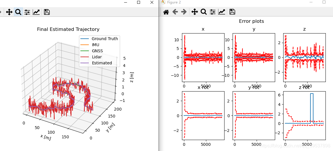
#### 6. Results and Analysis ###################################################################

################################################################################################
# Now that we have state estimates for all of our sensor data, let's plot the results. This plot
# will show the ground truth and the estimated trajectories on the same plot. Notice that the
# estimated trajectory continues past the ground truth. This is because we will be evaluating
# your estimated poses from the part of the trajectory where you don't have ground truth!
################################################################################################
est_traj_fig = plt.figure()
ax = est_traj_fig.add_subplot(111, projection='3d')
ax.plot(gt.p[:,0], gt.p[:,1], gt.p[:,2], label='Ground Truth')
ax.plot(gnss.data[:, 0], gnss.data[:, 1], gnss.data[:, 2], label="GNSS")
ax.plot(lidar.data[:, 0], lidar.data[:, 1], lidar.data[:, 2], label="Lidar")
ax.plot(p_est[:,0], p_est[:,1], p_est[:,2], label='Estimated')
ax.set_xlabel('x [m]')
ax.set_ylabel('y [m]')
ax.set_zlabel('z [m]')
ax.set_title('Final Estimated Trajectory')
ax.legend()
ax.set_zlim(-1, 5)
plt.show()

################################################################################################
# We can also plot the error for each of the 6 DOF, with estimates for our uncertainty
# included. The error estimates are in blue, and the uncertainty bounds are red and dashed.
# The uncertainty bounds are +/- 3 standard deviations based on our uncertainty.
################################################################################################
error_fig, ax = plt.subplots(2, 3)
error_fig.suptitle('Error plots')
num_gt = gt.p.shape[0]
p_est_euler = []

# Convert estimated quaternions to euler angles
for q in q_est:
    p_est_euler.append(Quaternion(*q).to_euler())
p_est_euler = np.array(p_est_euler)

# Get uncertainty estimates from P matrix
p_cov_diag_std = np.sqrt(np.diagonal(p_cov, axis1=1, axis2=2))

titles = ['x', 'y', 'z', 'x rot', 'y rot', 'z rot']
for i in range(3):
    ax[0, i].plot(range(num_gt), gt.p[:, i] - p_est[:num_gt, i])
    ax[0, i].plot(range(num_gt), 3 * p_cov_diag_std[:num_gt, i], 'r--')
    ax[0, i].plot(range(num_gt), -3 * p_cov_diag_std[:num_gt, i], 'r--')
    ax[0, i].set_title(titles[i])

for i in range(3):
    ax[1, i].plot(range(num_gt), gt.r[:, i] - p_est_euler[:num_gt, i])
    ax[1, i].plot(range(num_gt), 3 * p_cov_diag_std[:num_gt, i+6], 'r--')
    ax[1, i].plot(range(num_gt), -3 * p_cov_diag_std[:num_gt, i+6], 'r--')
    ax[1, i].set_title(titles[i+3])
plt.show()


#### 7. Submission #############################################################################

################################################################################################
# Now we can prepare your results for submission to the Coursera platform. Uncomment the
# corresponding lines to prepare a file that will save your position estimates in a format
# that corresponds to what we're expecting on Coursera.
################################################################################################

# Pt. 1 submission
'''
p1_indices = [9000, 9400, 9800, 10200, 10600]
p1_str = ''
for val in p1_indices:
    for i in range(3):
        p1_str += '%.3f ' % (p_est[val, i])
with open('pt1_submission.txt', 'w') as file:
    file.write(p1_str)
'''

# Pt. 2 submission
'''
p2_indices = [9000, 9400, 9800, 10200, 10600]
p2_str = ''
for val in p2_indices:
    for i in range(3):
        p2_str += '%.3f ' % (p_est[val, i])
with open('pt2_submission.txt', 'w') as file:
    file.write(p2_str)
'''

# Pt. 3 submission
'''
p3_indices = [6800, 7600, 8400, 9200, 10000]
p3_str = ''
for val in p3_indices:
    for i in range(3):
        p3_str += '%.3f ' % (p_est[val, i])
with open('pt3_submission.txt', 'w') as file:
    file.write(p3_str)
'''

结果图：