


根据李沐读论文学习一下这篇论文。
Transformer
Introduction
Recurrent neural networks, long short-term memory [13] and gated recurrent [7] neural networks in particular, have been firmly established as state of the art approaches in sequence modeling and transduction problems such as language modeling and machine translation [35, 2, 5]. Numerous efforts have since continued to push the boundaries of recurrent language models and encoder-decoder architectures [38, 24, 15]
在2017年语言转录问题的主要解决方法包括:RNN LSTM和GRNN。主流都是循环语言模型和编码器-解码器模型。
Recurrent models typically factor computation along the symbol positions of the input and output sequences. Aligning the positions to steps in computation time, they generate a sequence of hidden states ht, as a function of the previous hidden state ht−1 and the input for position t. This inherently sequential nature precludes parallelization within training xamples, which becomes critical at longer sequence lengths, as memory constraints limit batching across examples. Recent work has achieved significant improvements in computational efficiency through factorization tricks [21] and conditional computation [32], while also improving model performance in case of the latter. The fundamental constraint of sequential computation, however, remains.
RNN模型根据输入和输出序列的位置进行分解计算,由于它沿着时序依次计算,因此只有在前面部分完成后才能进行后面的计算,这就导致了两个问题:第一是难以进行GPU的并行计算,因此耗时长、计算性能差;第二是在很长的序列下,前面的信息在后续容易丢失,除非增加 h t h_t ht的大小,但是这又会导致计算开销较大。这些问题在研究中仍然存在。
Attention mechanisms have become an integral part of compelling sequence modeling and transduction models in various tasks, allowing modeling of dependencies without regard to their distance in the input or output sequences [2, 19]. In all but a few cases [27], however, such attention mechanisms are used in conjunction with a recurrent network.
Attention在当时的主要做法是与RNN结合使用,主要是解决如何将编码器的信息有效传给解码器的问题。
In this work we propose the Transformer, a model architecture eschewing recurrence and instead relying entirely on an attention mechanism to draw global dependencies between input and output.The Transformer allows for significantly more parallelization and can reach a new state of the art in
translation quality after being trained for as little as twelve hours on eight P100 GPUs.
提出的方法使用的是纯Attention网络,解决了并行处理问题,大大缩短计算时间。
Background
The goal of reducing sequential computation also forms the foundation of the Extended Neural GPU[16], ByteNet [18] and ConvS2S [9], all of which use convolutional neural networks as basic building block, computing hidden representations in parallel for all input and output positions. In these models,
the number of operations required to relate signals from two arbitrary input or output positions grows in the distance between positions, linearly for ConvS2S and logarithmically for ByteNet. This makes it more difficult to learn dependencies between distant positions [12]. In the Transformer this is
reduced to a constant number of operations, albeit at the cost of reduced effective resolution due to averaging attention-weighted positions, an effect we counteract with Multi-Head Attention as described in section 3.2.
利用CNN替代RNN进行并行计算的方法中,利用卷积将前后的信号联系起来,但是对于比较长序列,可能需要很多次卷积才能联系起来。而Transformer利用注意力机制就可以直接看到整个序列的情况。此外,CNN的输出是多个通道的,多通道的输出也可以当作是识别的多个模式,Transformer利用multi-head Attention来模拟多输出通道。
Self-attention, sometimes called intra-attention is an attention mechanism relating different positions of a single sequence in order to compute a representation of the sequence. Self-attention has been used successfully in a variety of tasks including reading comprehension, abstractive summarization, textual entailment and learning task-independent sentence representations [4, 27, 28, 22].
End-to-end memory networks are based on a recurrent attention mechanism instead of sequence-aligned recurrence and have been shown to perform well on simple-language question answering and language modeling tasks [34].
自注意力机制和memory network也是研究热点
To the best of our knowledge, however, the Transformer is the first transduction model relying entirely on self-attention to compute representations of its input and output without using sequence-aligned RNNs or convolution. In the following sections, we will describe the Transformer, motivate self-attention and discuss its advantages over models such as [17, 18] and [9].
Transformer是第一个仅仅依赖于自注意力机制来模拟encoder-decoder的。
Model Architecture
Most competitive neural sequence transduction models have an encoder-decoder structure [5, 2, 35].Here, the encoder maps an input sequence of symbol representations (x1, …, xn) to a sequence of continuous representations z = (z1, …, zn). Given z, the decoder then generates an output sequence (y1, …, ym) of symbols one element at a time. At each step the model is auto-regressive[10], consuming the previously generated symbols as additional input when generating the next.
encoder:将输入序列 ( x 1 , . . . , x n ) (x_1,...,x_n) (x1,...,xn)的每个单词映射为机器学习理解的向量 ( z 1 , . . . , z n ) (z_1,...,z_n) (z1,...,zn),encoder是一次性看整个句子的。
decoder:首先根据encoder 的输出得到输出序列 y 1 y_1 y1,然后根据 ( y 1 , . . . , y m − 1 ) (y_1,...,y_{m-1}) (y1,...,ym−1)得到 y m y_m ym,因此decoder是一个词往外输出的。并且decoder 属一种自回归模式(auto-regressive),它将过去时刻的输出作为当前时刻的输入。
The Transformer follows this overall architecture using stacked self-attention and point-wise, fully connected layers for both the encoder and decoder, shown in the left and right halves of Figure 1,respectively.
Transformer是由self-attention and point-wise, fully connected layers堆叠成的encoder和decoder。
Encoder and Decoder Stacks
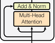
Encoder: The encoder is composed of a stack of N = 6 identical layers. Each layer has two sub-layers. The first is a multi-head self-attention mechanism, and the second is a simple, position wise fully connected feed-forward network. We employ a residual connection [11] around each of the two sub-layers, followed by layer normalization [1]. That is, the output of each sub-layer is LayerNorm(x + Sublayer(x)), where Sublayer(x) is the function implemented by the sub-layer itself. To facilitate these residual connections, all sub-layers in the model, as well as the embedding layers, produce outputs of dimension dmodel = 512.
encoder只有两个超参
N
=
6
N=6
N=6和
d
m
o
d
e
l
=
512
d_{model}=512
dmodel=512。
其中
N
=
6
N=6
N=6表示encoder由6个identical layers堆叠在一起,如下图红色方框所示:

每个layer都由两个子层构成,第一个子层是multi-head 自注意力机制,第二个子层就是简单的MLP。两个子层都使用了残差连接和layernorm。residual connections 需要输入输出维度一致,简单起见,固定每一层的输出维度512。(这样的做法在后面的Bert和GPT中被推广使用)
重点补充一下layernorm与batchnorm的区别:
对于二维样本(行为batch 列为feature时):
batchnorm是对一列数据进行标准化,而layernorm是对一行数据进行标准化。
对于三维样本(行为seq即
N
N
N 宽为feature即
d
m
o
d
e
l
d_{model}
dmodel 高为batch):

batchnorm:每次取一个特征,切一块(蓝色线),拉成一个向量,均值为 0 、方差为 1 的标准化。
layernorm:每次取一个样本,切一块(橙色线),拉成一个向量,均值为 0 、方差为 1 的标准化。
layernorm与batchnorm比起来,对于样本长度不相等的情况处理的更好。如果用batchnorm,对于样本长度不相等的,会自动填充0。对于Mini-batch 的均值和方差:如果样本长度变化比较大的时候,每次计算小批量的均值和方差,均值和方差的抖动大。对于全局的均值和方差:测试时遇到一个特别长的全新样本 (最上方蓝色阴影块),训练时未见过,训练时计算的均值和方差可能不好用。而layernorm每个样本自己算均值和方差,不需要存全局的均值和方差。
LayerNorm 和 BatchNorm 的例子理解:n 本书
BatchNorm:n本书,每本书的第一页拿出来,根据 n 本书的第一页的字数均值做 Norm。
LayerNorm:针对某一本书,这本书的每一页拿出来,根据次数每页的字数均值,自己做 Norm。
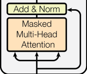
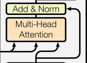
Decoder: The decoder is also composed of a stack of N = 6 identical layers. In addition to the two sub-layers in each encoder layer, the decoder inserts a third sub-layer, which performs multi-head attention over the output of the encoder stack. Similar to the encoder, we employ residual connections around each of the sub-layers, followed by layer normalization. We also modify the self-attention sub-layer in the decoder stack to prevent positions from attending to subsequent positions. This masking, combined with fact that the output embeddings are offset by one position, ensures that the predictions for position i can depend only on the known outputs at positions less than i.
decoder与encoder相比多了一个sub-layer,称为masked multi-head attention。decoder是自回归,之前时刻的输出是当前时刻的输入。但是attention一般能看到完整的输入。因此在做预测时,要利用mask掩盖t时刻之后的输入对t时刻的输出进行影响(保证训练和预测的行为一致)。(不让他看到本来应该由自己预测得到的东西)
Attention
An attention function can be described as mapping a query and a set of key-value pairs to an output, where the query, keys, values, and output are all vectors. The output is computed as a weighted sum of the values, where the weight assigned to each value is computed by a compatibility function of the query with the corresponding key.
注意力时将一个query和一组key-value映射为一个输出。输出是value的加权和,而权重根据query和每个value的相应的key的相似度进行计算。
对于同样的一组value-key,不同的query可以得到不同的权重,也就是不同的注意力机制。
Scaled Dot-Product Attention
We call our particular attention “Scaled Dot-Product Attention” (Figure 2). The input consists of
queries and keys of dimension dk, and values of dimension dv. We compute the dot products of the query with all keys, divide each by √dk, and apply a softmax function to obtain the weights on the values.
其实使用的是非常基础的注意力机制,它的输入由等长的queries和keys,长度均为 d k d_k dk和长度为 d v d_v dv的values组成,当然输出长度也会是 d v d_v dv。将query和keys做内积(内积越大代表相似度越大),然后除以 d k \sqrt{d_k} dk,最后利用softmax函数得到values的权重,softmax得到的权重非负并且和为1。
In practice, we compute the attention function on a set of queries simultaneously, packed together into a matrix Q. The keys and values are also packed together into matrices K and V . We compute the matrix of outputs as:
A t t e n t i o n ( Q , K , V ) = s o f t m a x ( Q ∗ K T / d k ) ∗ V Attention(Q, K, V ) = softmax(Q * K ^T / \sqrt{d_k})*V Attention(Q,K,V)=softmax(Q∗KT/dk)∗V
实际使用当中为了加速计算,会将query组成一个矩阵,通过矩阵的两次乘法进行并行计算。
假设Q为n行
d
k
d_k
dk列,K为m行
d
k
d_k
dk列,V为m行
d
v
d_v
dv列
Q
∗
K
T
Q * K ^T
Q∗KT得到的是n行m列,对于每一个query有一行key的内积值,然后除以
d
k
\sqrt{d_k}
dk后进行softmax计算,这样得到的也是每行独立的权重,也就是实现了多个query的并行计算。
然后与V相乘得到每行独立的权重结果。
The two most commonly used attention functions are additive attention [2], and dot-product (multiplicative) attention. Dot-product attention is identical to our algorithm, except for the scaling factor of √1\dk. Additive attention computes the compatibility function using a feed-forward network with a single hidden layer. While the two are similar in theoretical complexity, dot-product attention is much faster and more space-efficient in practice, since it can be implemented using highly optimized matrix multiplication code.
两种常见的注意力是加性注意力和内积注意力。该论文与内积注意力比较相似,只是加入了scaling的操作,选择这个是因为内积注意力的方法更快并且更加高效。
While for small values of dk the two mechanisms perform similarly, additive attention outperforms dot product attention without scaling for larger values of dk [3]. We suspect that for large values of dk, the dot products grow large in magnitude, pushing the softmax function into regions where it has extremely small gradients 4. To counteract this effect, we scale the dot products by √1\dk.
加入scale的操作是为了避免梯度消失。
在
d
k
\sqrt{d_k}
dk不大的时候,是否加入这个操作都没有什么影响。但是当
d
k
\sqrt{d_k}
dk较大的时候,也就是向量较长,内积可能非常大也可能非常小。当内积值较大时,差距也会较大,这样softmax的操作趋向于让大的更大,小的更小,也就是置信的地方更接近1,不置信的地方更接近0,由此得到收敛,因此梯度会很小。
而之前选择了
d
k
d_k
dk为512,所以还是要加入scale的操作。

mask的操作:保证 t 时刻的只看到 t 时刻以前的输入。通过将 t 时刻以后的Q和K的值替换成一个很大的负数,从而让 t 时刻以后的值经过softmax之后变成0。这样在计算权重的时候,t 时刻就只会用到
v
1
,
.
.
.
,
v
t
−
1
v_1,...,v_{t-1}
v1,...,vt−1的结果。
理解一下:mask时0 1矩阵,和attention的size一样,在 t 时刻以后的mask值为0。
Multi-head Attention
Instead of performing a single attention function with dmodel-dimensional keys, values and queries, we found it beneficial to linearly project the queries, keys and values h times with different, learned linear projections to dk, dk and dv dimensions, respectively. On each of these projected versions of queries, keys and values we then perform the attention function in parallel, yielding dv-dimensional output values. These are concatenated and once again projected, resulting in the final values, as depicted in Figure 2.
multi-head Attention与简单的attention不同,它首先将queries, keys 和 values投影h次,得到维度为
d
k
,
d
k
d_k, d_k
dk,dk和
d
v
d_v
dv。然后分别同时进行Scaled Dot-Product Attention,最后将结果连接起来,再进行一次投影得到最终结果,如下图所示:

选择multi-head的原因是,简单的内积attention可调参数基本没有,因此通过投影h次来让模型识别不同的模式,有点类似于CNN的多通道操作。
具体表达式如下:
M
u
l
t
i
H
e
a
d
(
Q
,
K
,
V
)
=
C
o
n
c
a
t
(
h
e
a
d
1
,
.
.
.
,
h
e
a
d
h
)
W
O
MultiHead(Q, K, V ) = Concat(head_1, ..., head_h)W^O
MultiHead(Q,K,V)=Concat(head1,...,headh)WO
w
h
e
r
e
:
h
e
a
d
i
=
A
t
t
e
n
t
i
o
n
(
Q
i
W
,
K
i
W
,
V
i
W
)
where:head_i = Attention(Q^W_i, K^W_i, V^W_i)
where:headi=Attention(QiW,KiW,ViW)
Applications of Attention in our Model
Transformer当中有三种模式的Attention。
第一种是encoder里面的Attention:
The encoder contains self-attention layers. In a self-attention layer all of the keys, values and queries come from the same place, in this case, the output of the previous layer in the encoder. Each position in the encoder can attend to all positions in the previous layer of the encoder.
如下图所示,从左到右输入依次是V K Q,因此在编码器的V=K=Q,也称为self-attention。假设不存在multi-head,v为n个长度为d的向量,那么输出也会是n个长度为d的向量,并且输出的每一个向量
o
u
t
t
out_t
outt都是:每个输入向量
v
t
v_t
vt与所有向量
v
v
v的相似度作为加权计算得到(query=value=key的结果)。然后在multi-head的模式下,会得到h个不同的映射。
第二种是decoder里面的Attention:
Similarly, self-attention layers in the decoder allow each position in the decoder to attend to all positions in the decoder up to and including that position. We need to prevent leftward information flow in the decoder to preserve the auto-regressive property. We implement this inside of scaled dot-product attention by masking out (setting to −∞) all values in the input of the softmax which correspond to illegal connections. See Figure 2
decoder也是self-attention,但是它使用了mask来保证 t 时刻的输出只会受到 t 时刻之前的输入的影响,也就是利用 mask 将 t 时刻以后的值设为负无穷。
第三种是encoder-decoder里面的attention:
In “encoder-decoder attention” layers, the queries come from the previous decoder layer, and the memory keys and values come from the output of the encoder. This allows every position in the decoder to attend over all positions in the input sequence. This mimics the typical encoder-decoder attention mechanisms in sequence-to-sequence models such as[38, 2, 9].
该attention的V和K来自于encoder的输出(长度为n),Q来自于decoder的输出(长度为m),然按照attention的规则,对于每一个query,依次比较其与K的相似度,将其作为V的加权
Position-wise Feed-Forward Networks
In addition to attention sub-layers, each of the layers in our encoder and decoder contains a fully connected feed-forward network, which is applied to each position separately and identically. This consists of two linear transformations with a ReLU activation in between.
F F N ( x ) = m a x ( 0 , x W 1 + b 1 ) W 2 + b 2 FFN(x) = max(0, xW_1 + b_1)W_2 + b_2 FFN(x)=max(0,xW1+b1)W2+b2
While the linear transformations are the same across different positions, they use different parameters from layer to layer. Another way of describing this is as two convolutions with kernel size 1.The dimensionality of input and output is dmodel = 512, and the inner-layer has dimensionality df = 2048.
实际上这就是一个MLP,但是它是对每个词单独作用,并且保证对不同词作用的MLP参数相同。因此FFN实际就是一个线性层加上一个ReLU再加上一个线性层。
单隐藏层的 MLP,中间
W
1
W_1
W1 扩维到4倍 2048,最后
W
2
W_2
W2 投影回到 512 维度大小,便于残差连接。
比较Transformer和RNN的作用方式:
Transformer首先利用Attention将整个序列的有用信息汇聚起来,后面的MLP只需对每个点独立作用,因为每个点都已经利用attention汇聚了它感兴趣的部分。
因此Transformer是先全局提取序列信息然后利用MLP进行语义转换,而RNN是每次将上一时刻的信息输入到下一时刻。

Embeddings and Softmax
Similarly to other sequence transduction models, we use learned embeddings to convert the input tokens and output tokens to vectors of dimension dmodel. We also use the usual learned linear transformation and softmax function to convert the decoder output to predicted next-token probabilities. In our model, we share the same weight matrix between the two embedding layers and the pre-softmax linear transformation, similar to [30]. In the embedding layers, we multiply those weights by √dmodel.
在encoder和decoder和pre-softmax的三者之前都加入了embedding,并且享受相同的权重。
Positional Encoding
attention的输出结果仅仅是加权和,不包含有顺序信息,因此需要加入位置信息。


 被折叠的 条评论
为什么被折叠?
被折叠的 条评论
为什么被折叠?
 到【灌水乐园】发言


