机器学习——集成学习进阶

XGBoost

极端梯度提升树

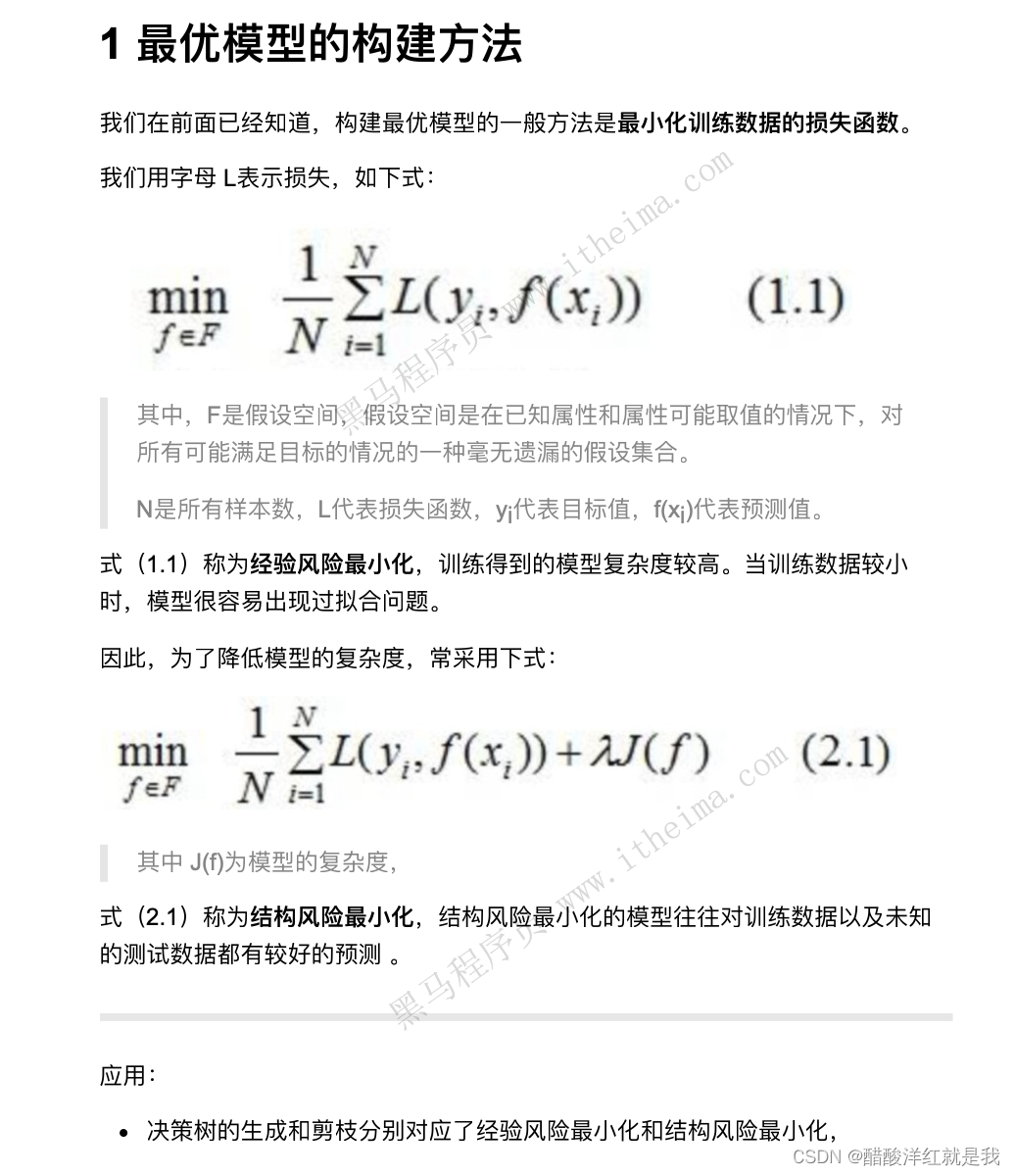
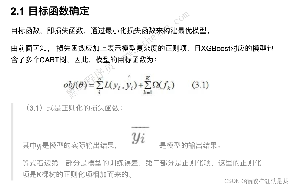
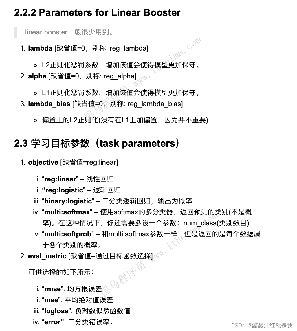
目标函数

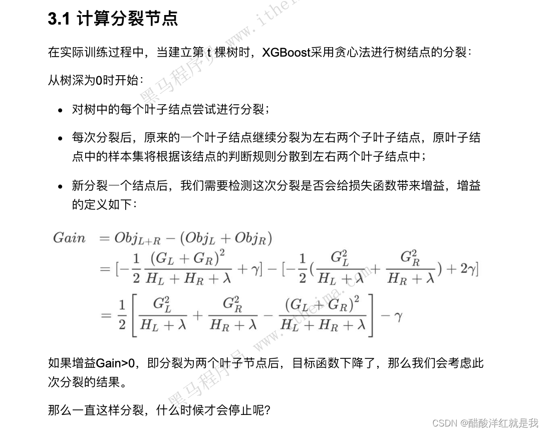
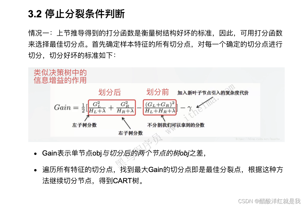
XGBoost回归树构建方法

XGboost和GDBT的区别

api介绍

XGBoost案例

在决策树中的机器学习部分代码进行修改

# 4.xgboost模型训练
# 4.1 初步模型训练
from xgboost import XGBClassifier

xg = XGBClassifier()

xg.fit(x_train, y_train)

xg.score(x_test, y_test)

0.7832699619771863

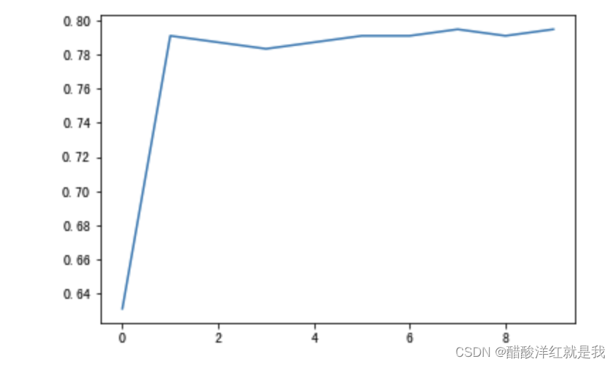
# 4.2 对max_depth进行调优

depth_range  = range(10)
score = []

for i in depth_range:
    xg = XGBClassifier(eta=1, gamma=0, max_depth=i)
    xg.fit(x_train, y_train)
    
    s = xg.score(x_test, y_test)
    
    print(s)
    score.append(s)

0.6311787072243346
0.7908745247148289
0.7870722433460076
0.7832699619771863
0.7870722433460076
0.7908745247148289
0.7908745247148289
0.7946768060836502
0.7908745247148289
0.7946768060836502

# 4.3 调优结果可视化
import matplotlib.pyplot as plt

plt.plot(depth_range, score)

plt.show()

otto案例——xgboost实现

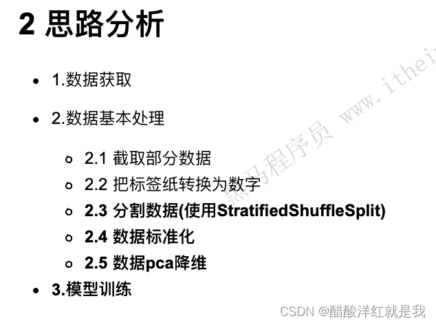
# 通过StratifiedShuffleSplit实现数据分割

from sklearn.model_selection import StratifiedShuffleSplit

sss = StratifiedShuffleSplit(n_splits=1, test_size=0.2, random_state=0)

for train_index, test_index in sss.split(X_resampled.values, y_resampled):
    print(len(train_index))
    print(len(test_index))
    
    x_train = X_resampled.values[train_index]
    x_val = X_resampled.values[test_index]
    
    y_train = y_resampled[train_index]
    y_val = y_resampled[test_index]

#数据标准化
from sklearn.preprocessing import StandardScaler

scaler = StandardScaler()
scaler.fit(x_train)

x_train_scaled = scaler.transform(x_train)
x_val_scaled = scaler.transform(x_val)

#数据PCA降维
from sklearn.decomposition import PCA

pca = PCA(n_components=0.9)

x_train_pca = pca.fit_transform(x_train_scaled)
x_val_pca = pca.transform(x_val_scaled)

# 可视化数据降维信息变化程度
plt.plot(np.cumsum(pca.explained_variance_ratio_))

plt.xlabel("元素数量")
plt.ylabel("表达信息百分占比")

plt.show()

#基本模型训练
from xgboost import XGBClassifier

xgb = XGBClassifier()
xgb.fit(x_train_pca, y_train)

# 输出预测值,一定输出带有百分占比的预测值
y_pre_proba = xgb.predict_proba(x_val_pca)

# logloss评估
from sklearn.metrics import log_loss
log_loss(y_val, y_pre_proba, eps=1e-15, normalize=True)

xgb.get_params

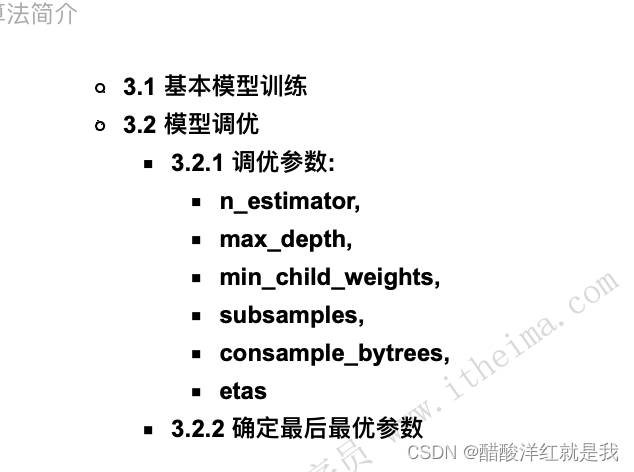
#模型调优
#确定最优的estimators
scores_ne = []
n_estimators = [100, 200, 300, 400, 500, 550, 600, 700]

for nes in n_estimators:
    print("n_estimators:", nes)
    xgb = XGBClassifier(max_depth=3,
                        learning_rate=0.1, 
                        n_estimators=nes, 
                        objective="multi:softprob", 
                        n_jobs=-1, 
                        nthread=4, 
                        min_child_weight=1,
                        subsample=1,
                        colsample_bytree=1,
                        seed=42)
    
    xgb.fit(x_train_pca, y_train)
    y_pre = xgb.predict_proba(x_val_pca)
    score = log_loss(y_val, y_pre)
    scores_ne.append(score)
    
    print("每次测试的logloss值是:{}".format(score))

# 图形化展示相应的logloss值
plt.plot(n_estimators, scores_ne, "o-")

plt.xlabel("n_estimators")
plt.ylabel("log_loss")
plt.show()

print("最优的n_estimators值是:{}".format(n_estimators[np.argmin(scores_ne)]))

#确定最优的max_depth
scores_md = []
max_depths = [1,3,5,6,7]

for md in max_depths:
    print("max_depth:", md)
    xgb = XGBClassifier(max_depth=md,
                        learning_rate=0.1, 
                        n_estimators=n_estimators[np.argmin(scores_ne)], 
                        objective="multi:softprob", 
                        n_jobs=-1, 
                        nthread=4, 
                        min_child_weight=1,
                        subsample=1,
                        colsample_bytree=1,
                        seed=42)
    
    xgb.fit(x_train_pca, y_train)
    y_pre = xgb.predict_proba(x_val_pca)
    score = log_loss(y_val, y_pre)
    scores_md.append(score)
    
    print("每次测试的logloss值是:{}".format(score))

# 图形化展示相应的logloss值
plt.plot(max_depths, scores_md, "o-")

plt.xlabel("max_depths")
plt.ylabel("log_loss")
plt.show()

print("最优的max_depths值是:{}".format(max_depths[np.argmin(scores_md)]))

#确定最佳参数
xgb = XGBClassifier(learning_rate =0.1, 
                    n_estimators=550, 
                    max_depth=3, 
                    min_child_weight=3, 
                    subsample=0.7, 
                    colsample_bytree=0.7, 
                    nthread=4, 
                    seed=42, 
                    objective='multi:softprob')

xgb.fit(x_train_scaled, y_train)

y_pre = xgb.predict_proba(x_val_scaled)

print("测试数据的log_loss值为 : {}".format(log_loss(y_val, y_pre, eps=1e-15, normalize=True)))

lightGBM

主要基于以下方面优化，提升整体特性：

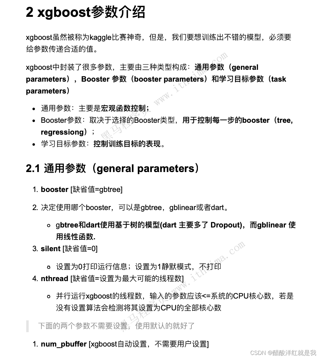
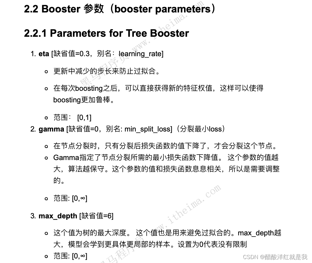
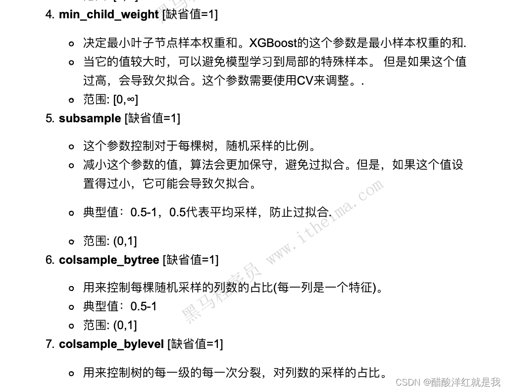
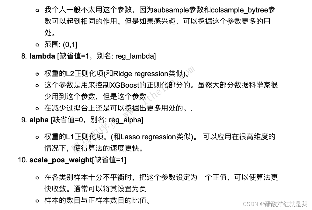
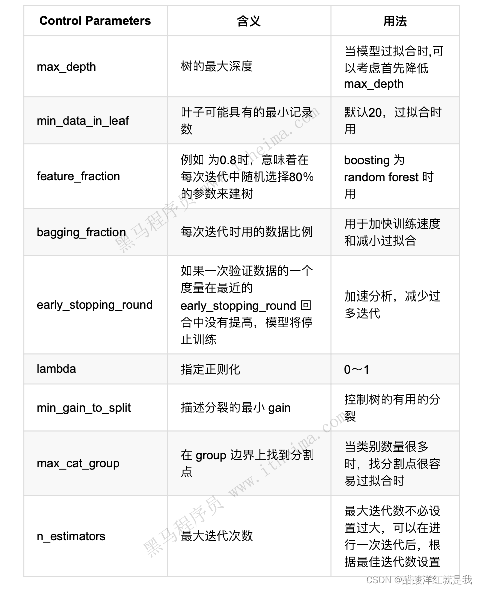
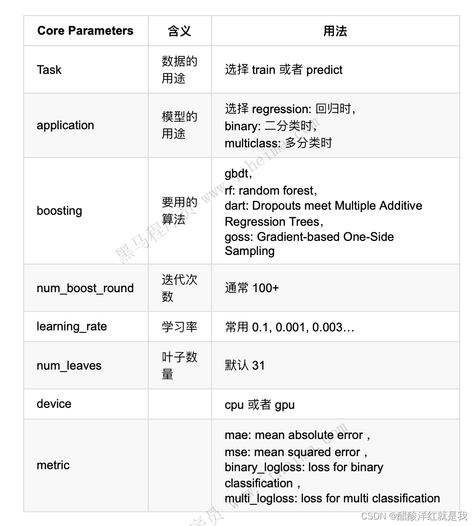
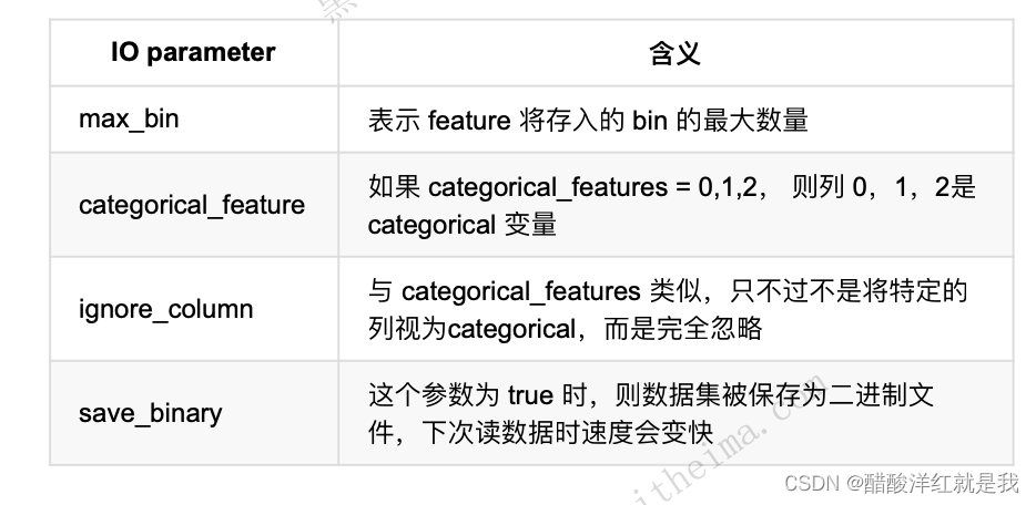
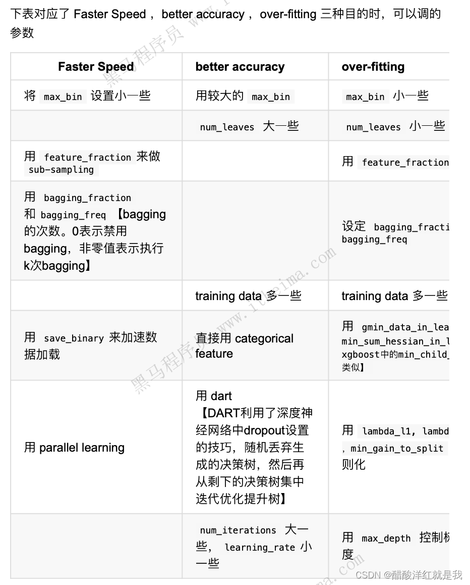
参数介绍

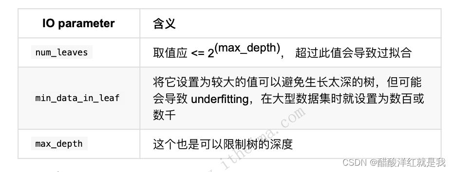
调参建议

lightGBM案例

from sklearn.datasets import load_iris
from sklearn.model_selection import train_test_split
from sklearn.model_selection import GridSearchCV
from sklearn.metrics import mean_squared_error
import lightgbm as lgb

#读取数据
iris = load_iris()
data = iris.data
target = iris.target

#数据基本处理
X_train, X_test, y_train, y_test = train_test_split(data, target, test_size=0.2)

#模型训练
#模型基本训练
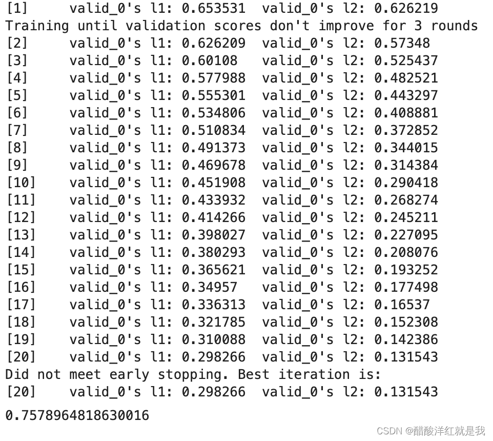
gbm = lgb.LGBMRegressor(objective="regression", learning_rate=0.05, n_estimators=20)

gbm.fit(X_train, y_train, eval_set=[(X_test, y_test)], eval_metric="l1", early_stopping_rounds=3)
gbm.score(X_test, y_test)

#通过网格搜索进行训练
estimators = lgb.LGBMRegressor(num_leaves=31)
param_grid = {
    "learning_rate": [0.01, 0.1, 1],
    "n_estmators":[20, 40, 60, 80]
}
gbm = GridSearchCV(estimators, param_grid, cv=5)
gbm.fit(X_train, y_train)

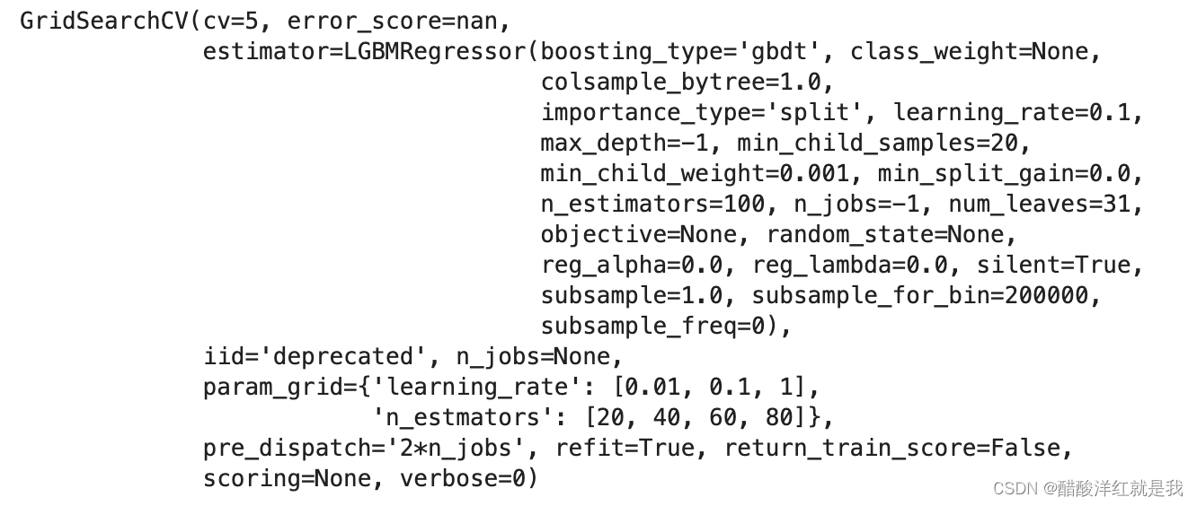
gbm.best_params_

{‘learning_rate’: 0.1, ‘n_estmators’: 20}

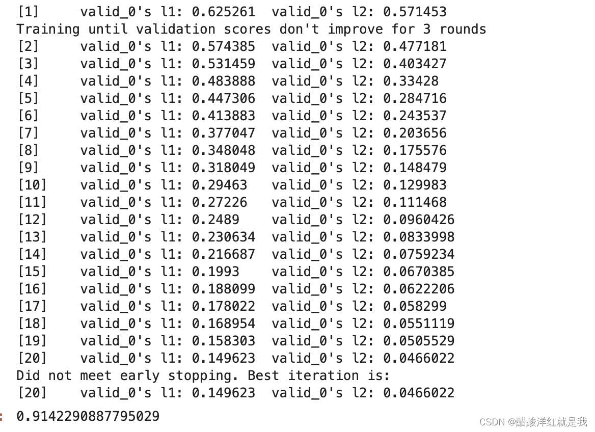
gbm = lgb.LGBMRegressor(objective="regression", learning_rate=0.1, n_estimators=20)

gbm.fit(X_train, y_train, eval_set=[(X_test, y_test)], eval_metric="l1", early_stopping_rounds=3)
gbm.score(X_test, y_test)

《绝地求生》玩家排名预测

import numpy as np
import matplotlib.pyplot as plt
import pandas as pd
import seaborn as sns
train = pd.read_csv("./data/train_V2.csv")

#数据基本处理
#数据缺失值处理
# 判断哪列有缺失值,发现只有winPlacePerc有 
np.any(train.isnull())

# 查找缺失值
train[train["winPlacePerc"].isnull()]

# 删除
train = train.drop(2744604)

#特征数据规范化处理
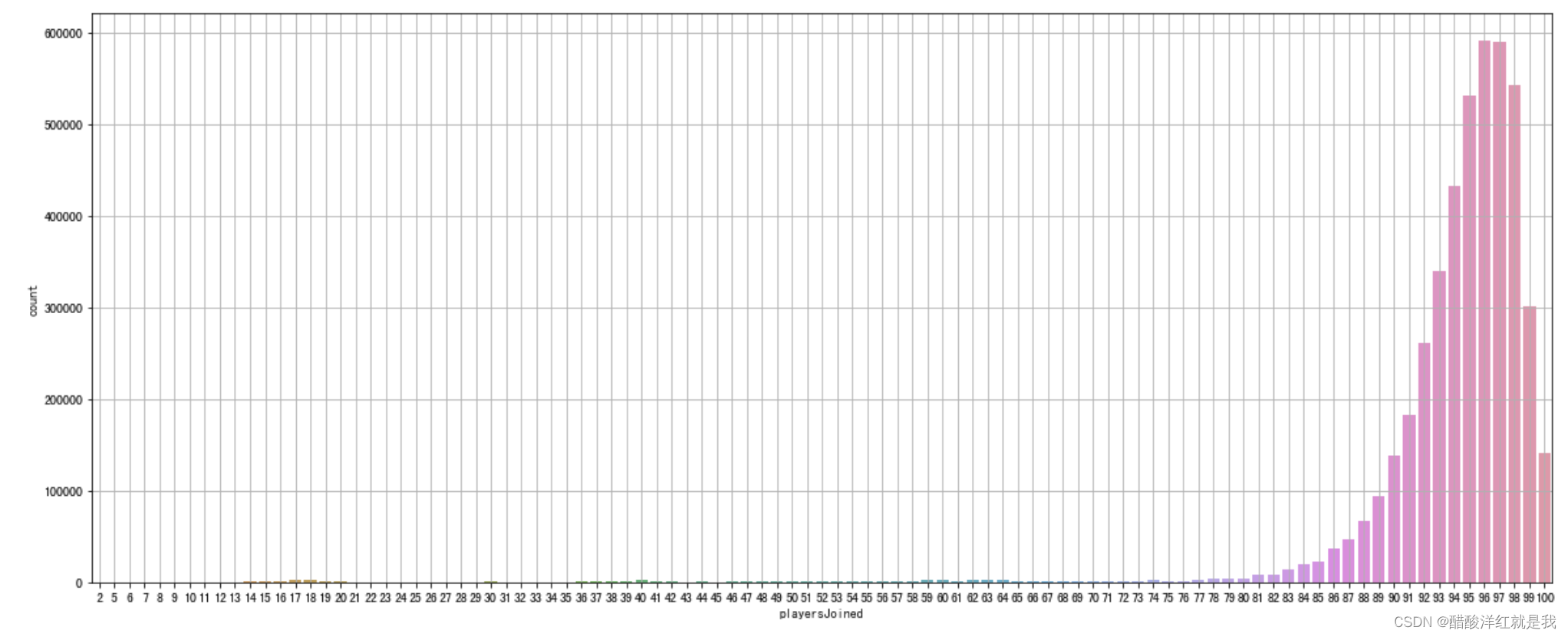
#查看每场比赛参加的人数
count = train.groupby("matchId")["matchId"].transform("count")

train["playersJoined"] = count
train["playersJoined"].sort_values()

plt.figure(figsize=(20, 8))
sns.countplot(train["playersJoined"])
plt.grid()
plt.show()

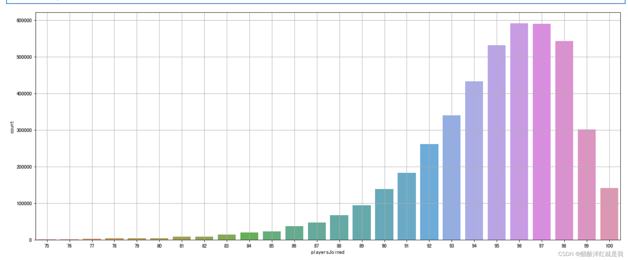
plt.figure(figsize=(20, 8))
sns.countplot(train[train["playersJoined"]>=75]["playersJoined"])
plt.grid()
plt.show()

#规范化输出部分数据
train["killsNorm"] = train["kills"] * ((100-train["playersJoined"])/100+1)
train["damageDealtNorm"] = train["damageDealt"] * ((100-train["playersJoined"])/100+1)
train["maxPlaceNorm"] = train["maxPlace"] * ((100-train["playersJoined"])/100+1)
train["matchDurationNorm"] = train["matchDuration"] * ((100-train["playersJoined"])/100+1)

# 比较经过规范化的特征值和原始特征值的值
to_show = ['Id', 'kills','killsNorm','damageDealt', 'damageDealtNorm', 'maxPlace', 'maxPlaceNorm', 'matchDuration', 'matchDurationNorm']
train[to_show][0:11]

#部分变量合成
train["healsandboosts"] = train["heals"] + train["boosts"]

#异常值处理
#异常值处理：删除有击杀，但是完全没有移动的玩家
train["totalDistance"] = train["rideDistance"] + train["walkDistance"] + train["swimDistance"]
train["killwithoutMoving"] = (train["kills"] > 0) & (train["totalDistance"] == 0)
train.drop(train[train["killwithoutMoving"] == True].index, inplace=True)

#异常值处理：删除驾车杀敌数异常的数据
train.drop(train[train["roadKills"] > 10].index, inplace=True)

#异常值处理：删除玩家在一局中杀敌数超过30人的数据
train.drop(train[train["kills"] > 30].index, inplace=True)

#异常值处理：删除爆头率异常数据
train["headshot_rate"] = train["headshotKills"]/train["kills"]
train["headshot_rate"] = train["headshot_rate"].fillna(0)
train.drop(train[(train["headshot_rate"] == 1) & (train["kills"] > 9)].index, inplace=True)

#异常值处理：删除最远杀敌距离异常数据
train.drop(train[train["longestKill"] >=1000].index, inplace=True)

#异常值处理：删除关于运动距离的异常值
train.drop(train[train["walkDistance"] >=10000].index, inplace=True)
train.drop(train[train["rideDistance"] >=20000].index, inplace=True)
train.drop(train[train["swimDistance"] >=20000].index, inplace=True)

#异常值处理：武器收集异常值处理
train.drop(train[train["weaponsAcquired"] >=80].index, inplace=True)

#异常值处理：删除使用治疗药品数量异常值
train.drop(train[train["heals"] >=80].index, inplace=True)

#类别型数据处理
#比赛类型one-hot处理
train["matchType"].unique()
train = pd.get_dummies(train, columns=["matchType"])
matchType_encoding = train.filter(regex="matchType")

#对groupId,matchId等数据进行处理
train["groupId"] = train["groupId"].astype("category")
train["groupId_cat"] = train["groupId"].cat.codes
train["matchId"] = train["matchId"].astype("category")
train["matchId_cat"] = train["matchId"].cat.codes
train.drop(["groupId", "matchId"], axis=1, inplace=True)

#数据截取
#取部分数据进行使用（100000）
df_sample = train.sample(100000)

#确定特征值和目标值
df = df_sample.drop(["winPlacePerc", "Id"], axis=1)

y = df_sample["winPlacePerc"]   

#分割训练集和测试集
from sklearn.model_selection import train_test_split
X_train, X_valid, y_train, y_valid = train_test_split(df, y, test_size=0.2)

#机器学习（模型训练）和评估
from sklearn.ensemble import RandomForestRegressor
from sklearn.metrics import mean_absolute_error

#使用随机森林对模型进行训练
#初步使用随机森林进行模型训练
m1 = RandomForestRegressor(n_estimators=40, 
                           min_samples_leaf=3, 
                           max_features='sqrt',
                           n_jobs=-1)

m1.fit(X_train, y_train)

y_pre = m1.predict(X_valid)
m1.score(X_valid, y_valid)
mean_absolute_error(y_valid, y_pre)

#再次使用随机森林，进行模型训练
m1.feature_importances_
imp_df = pd.DataFrame({"cols":df.columns, "imp":m1.feature_importances_})
imp_df = imp_df.sort_values("imp", ascending=False)
imp_df[:20].plot("cols", "imp", figsize=(20, 8), kind="barh")

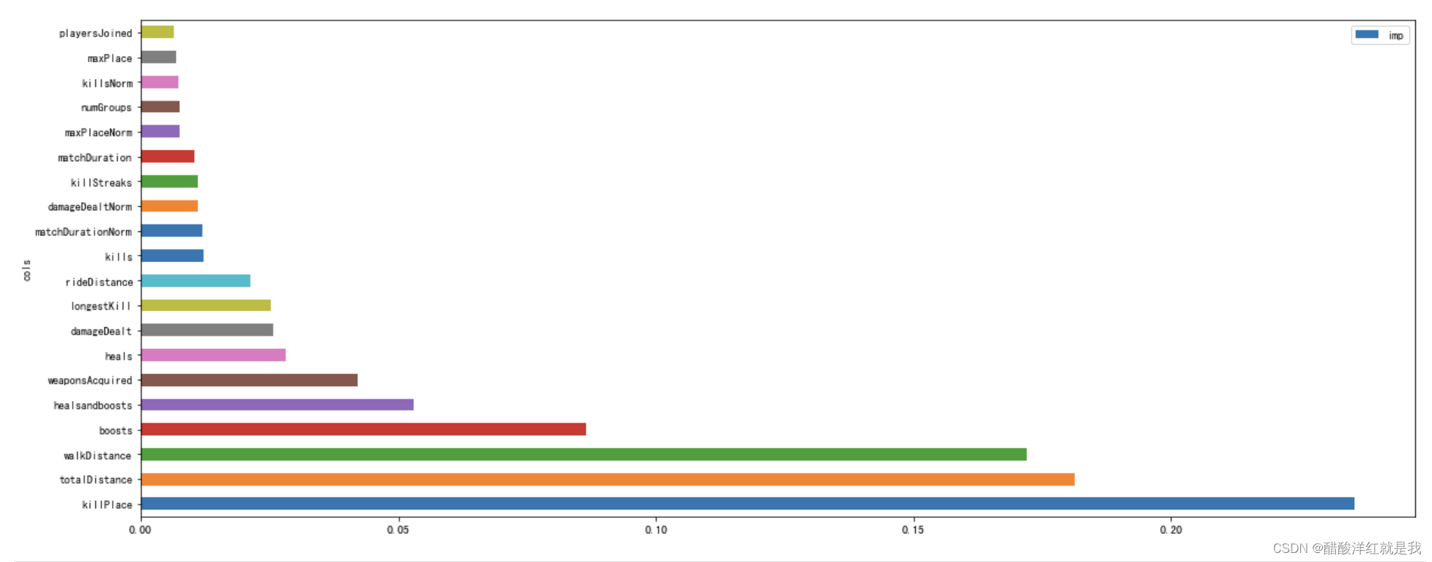
to_keep = imp_df[imp_df.imp > 0.005].cols
df_keep = df[to_keep]
X_train, X_valid, y_train, y_valid = train_test_split(df_keep, y, test_size=0.2)
m2 = RandomForestRegressor(n_estimators=40, 
                           min_samples_leaf=3, 
                           max_features='sqrt',
                           n_jobs=-1)

m2.fit(X_train, y_train)

y_pre = m2.predict(X_valid)
m2.score(X_valid, y_valid)
mean_absolute_error(y_valid, y_pre)

#使用lightGBM对模型进行训练
X_train, X_valid, y_train, y_valid = train_test_split(df, y, test_size=0.2)

#模型初次尝试
import lightgbm as lgb
gbm = lgb.LGBMRegressor(objective="regression", num_leaves=31, learning_rate=0.05, n_estimators=20)

gbm.fit(X_train, y_train, eval_set=[(X_valid, y_valid)], eval_metric="l1", early_stopping_rounds=5)

y_pre = gbm.predict(X_valid, num_iteration=gbm.best_iteration_)
mean_absolute_error(y_valid, y_pre)

#模型二次调优
from sklearn.model_selection import GridSearchCV
estimator = lgb.LGBMRegressor(num_leaves=31)
param_grid = {
    "learning_rate":[0.01, 0.1, 1],
    "n_estimators":[40, 60, 80, 100, 200, 300]
}

gbm = GridSearchCV(estimator, param_grid, cv=5, n_jobs=-1)

gbm.fit(X_train, y_train)

y_pre = gbm.predict(X_valid)
mean_absolute_error(y_valid, y_pre)
gbm.best_params_

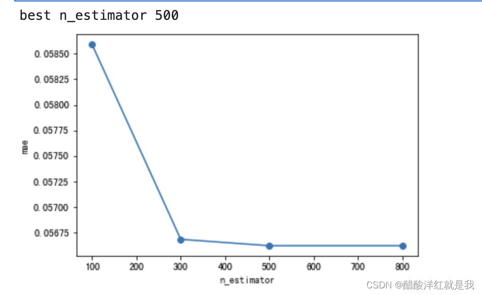
#模型三次调优
# n_estimators

scores = []
n_estimators = [100, 300, 500, 800]

for nes in  n_estimators:
    lgbm = lgb.LGBMRegressor(boosting_type='gbdt', 
                      num_leaves=31,
                      max_depth=5,
                      learning_rate=0.1,
                      n_estimators=nes,
                      min_child_samples=20,
                      n_jobs=-1)
    
    lgbm.fit(X_train, y_train, eval_set=[(X_valid, y_valid)], eval_metric="l1", early_stopping_rounds=5)
    
    y_pre = lgbm.predict(X_valid)
    
    mae = mean_absolute_error(y_valid, y_pre)
    
    scores.append(mae)
    print("本次结果输出的mae值是:\n", mae)

plt.plot(n_estimators,scores,'o-')
plt.ylabel("mae")
plt.xlabel("n_estimator")
print("best n_estimator {}".format(n_estimators[np.argmin(scores)]))

# max_depth

scores = []
max_depth = [3, 5, 7, 9, 11]

for md in  max_depth:
    lgbm = lgb.LGBMRegressor(boosting_type='gbdt', 
                      num_leaves=31,
                      max_depth=md,
                      learning_rate=0.1,
                      n_estimators=500,
                      min_child_samples=20,
                      n_jobs=-1)
    
    lgbm.fit(X_train, y_train, eval_set=[(X_valid, y_valid)], eval_metric="l1", early_stopping_rounds=5)
    
    y_pre = lgbm.predict(X_valid)
    
    mae = mean_absolute_error(y_valid, y_pre)
    
    scores.append(mae)
    print("本次结果输出的mae值是:\n", mae)

plt.plot(max_depth,scores,'o-')
plt.ylabel("mae")
plt.xlabel("max_depths")
print("best max_depths {}".format(max_depth[np.argmin(scores)]))

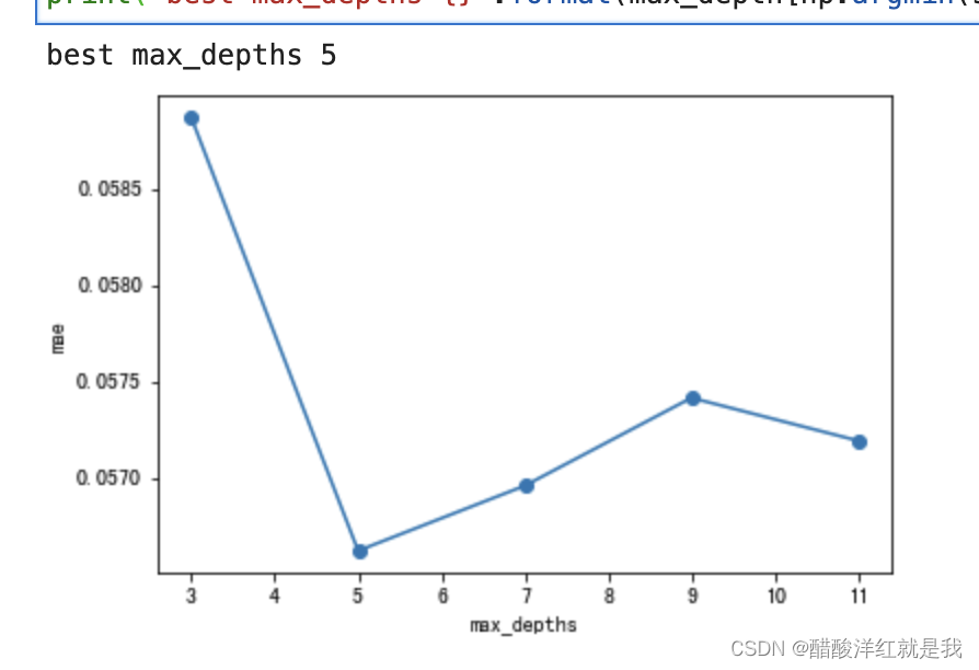
scores

[0.058867698663447106,
0.0566209902947507,
0.05695850296967709,
0.057414793402343275,
0.0571923061736829]