记录|深度学习100例-卷积神经网络（CNN）服装图像分类 | 第3天

记录|深度学习100例-卷积神经网络（CNN）服装图像分类 | 第3天

1. 服装图像分类效果图

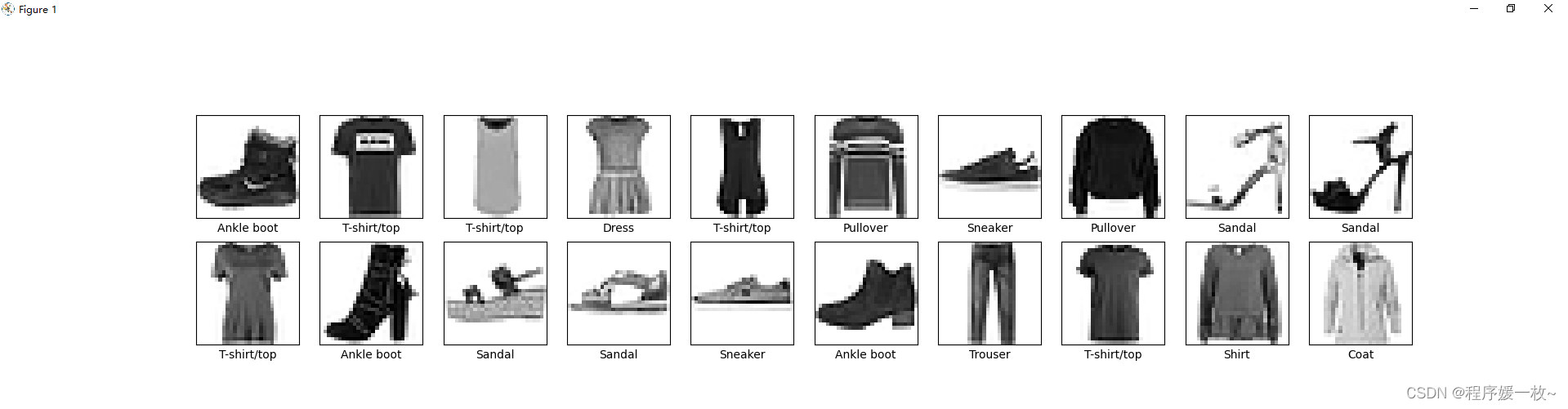
原始训练图如下：

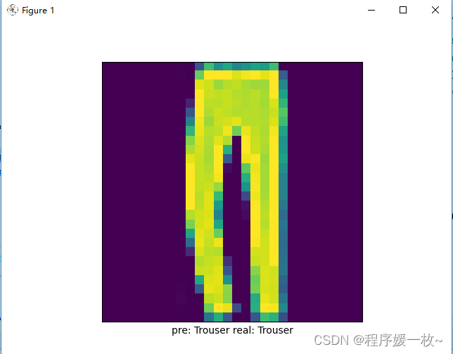
测试图：预测标签及实际标签如下：
可以看到正确预测

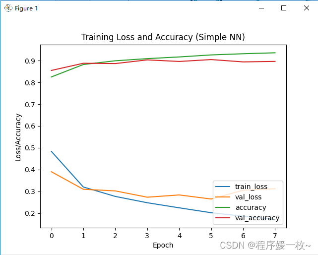
训练损失/准确度图：

2. 源码

# 深度学习100例-卷积神经网络（CNN）服装图像分类 | 第3天
# USAGE
# python img_fashion3.py

import matplotlib.pyplot as plt
import numpy as np
import tensorflow as tf
from tensorflow.keras import datasets, layers, models

gpus = tf.config.list_physical_devices("GPU")

if gpus:
    gpu0 = gpus[0]  # 如果有多个GPU，仅使用第0个GPU
    tf.config.experimental.set_memory_growth(gpu0, True)  # 设置GPU显存用量按需使用
    tf.config.set_visible_devices([gpu0], "GPU")

# 导入数据
(train_images, train_labels), (test_images, test_labels) = datasets.fashion_mnist.load_data()

# 将像素的值标准化至0到1的区间内。
train_images, test_images = train_images / 255.0, test_images / 255.0

# 调整数据到我们需要的格式
train_images = train_images.reshape((60000, 28, 28, 1))
test_images = test_images.reshape((10000, 28, 28, 1))
print(train_images.shape, test_images.shape, train_labels.shape, test_labels.shape)

# class_names = ['T恤/上衣', '裤子', '套头衫', '连衣裙', '外套','凉鞋', '衬衫', '运动鞋', '包', '短靴']
class_names = ['T-shirt/top', 'Trouser', 'Pullover', 'Dress', 'Coat',
               'Sandal', 'Shirt', 'Sneaker', 'Bag', 'Ankle boot']

# 可视化
plt.figure(figsize=(20, 10))
for i in range(20):
    plt.subplot(5, 10, i + 1)
    plt.xticks([])
    plt.yticks([])
    plt.grid(False)
    plt.imshow(train_images[i], cmap=plt.cm.binary)
    plt.xlabel(class_names[train_labels[i]])
plt.show()

# 构建网络
model = models.Sequential([
    layers.Conv2D(32, (3, 3), activation='relu', input_shape=(28, 28, 1)),  # 卷积层1，卷积核3*3
    layers.MaxPooling2D((2, 2)),  # 池化层1，2*2采样
    layers.Conv2D(64, (3, 3), activation='relu'),  # 卷积层2，卷积核3*3
    layers.MaxPooling2D((2, 2)),  # 池化层2，2*2采样
    layers.Conv2D(64, (3, 3), activation='relu'),  # 卷积层3，卷积核3*3

    layers.Flatten(),  # Flatten层，连接卷积层与全连接层
    layers.Dense(64, activation='relu'),  # 全连接层，特征进一步提取
    layers.Dense(10)  # 输出层，输出预期结果
])

model.summary()  # 打印网络结构

# 编译模型
model.compile(optimizer='adam',
              loss=tf.keras.losses.SparseCategoricalCrossentropy(from_logits=True),
              metrics=['accuracy'])

# 训练模型
history = model.fit(train_images, train_labels, epochs=8,
                    validation_data=(test_images, test_labels))

pre = model.predict(test_images)
print('pre: ' + str(class_names[np.argmax(pre[2])]) + ' real: ' + str(class_names[test_labels[2]]))

plt.imshow(test_images[2])
plt.xticks([])
plt.yticks([])
plt.xlabel('pre: ' + class_names[np.argmax(pre[2])] + ' real: ' + str(class_names[test_labels[2]]))
plt.show()

plt.plot(history.history["loss"], label="train_loss")
plt.plot(history.history["val_loss"], label="val_loss")
plt.plot(history.history['accuracy'], label='accuracy')
plt.plot(history.history['val_accuracy'], label='val_accuracy')
plt.title("Training Loss and Accuracy (Simple NN)")
plt.xlabel('Epoch')
plt.ylabel('Loss/Accuracy')
# plt.ylim([0.5, 1])
plt.legend(loc='lower right')
plt.show()

test_loss, test_acc = model.evaluate(test_images, test_labels, verbose=2)
print(test_acc)

参考

• https://mtyjkh.blog.csdn.net/article/details/116992196