


转载自:概念
概念
分支定界算法始终围绕着一颗搜索树进行的,我们将原问题看作搜索树的根节点,从这里出发,分支的含义就是将大的问题分割成小的问题。
大问题可以看成是搜索树的父节点,那么从大问题分割出来的小问题就是父节点的子节点了。
分支的过程就是不断给树增加子节点的过程。而定界就是在分支的过程中检查子问题的上下界,如果子问题不能产生一比当前最优解还要优的解,那么砍掉这一支。直到所有子问题都不能产生一个更优的解时,算法结束。
原理
对于一个整数规划模型
因为求解的是最大化问题,我们不妨设当前的最优解BestV为-INF,表示负无穷。

通过线性松弛求得两个子问题的upper bound为Z_LP1 = 12.75,Z_LP2 = 12.2。由于Z_LP1 和Z_LP2都大于BestV=-INF,说明这两支有机会出现最优解。继续往下。
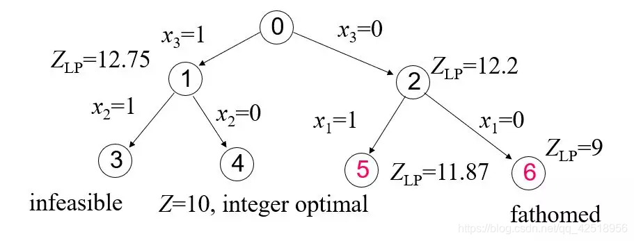
子问题3已经不可行,无需再理。
子问题4通过线性松弛得到最优解为10,刚好也符合原问题0的所有约束,在该支找到一个可行解,更新BestV = 10。
子问题5通过线性松弛得到upper bound为11.87 > 当前的BestV = 10,因此子问题5还有戏,待下一次分支。
子问题6得到upper bound为9 < 当前的BestV = 10,那么从该支下去找到的解也不会变得更好,所以剪掉!

子问题7不可行,无需再理。
子问题8得到一个满足原问题0所有约束的解,但是目标值为4<当前的BestV=10,所以不更新BestV,同时该支下去也不能得到更好的解了。

分支定界法(branch and bound)是一种求解整数规划问题的最常用算法。这种方法不但可以求解纯整数规划,还可以求解混合整数规划问题。
1. Using a heuristic, find a solution xh to the optimization problem. Store its value, B = f(x_h). (If no heuristic is available, set B to infinity.) B will denote the best solution found so far, and will be used as an upper bound on candidate solutions.

2. Initialize a queue to hold a partial solution with none of the variables of the problem assigned.

3. Loop until the queue is empty:

    3.1. Take a node N off the queue.

    3.2. If N represents a single candidate solution x and f(x) < B, then x is the best solution so far. Record it and set B ← f(x).

    3.3. Else, branch on N to produce new nodes Ni. For each of these:

        3.3.1. If bound(N_i) > B, do nothing; since the lower bound on this node is greater than the upper bound of the problem, it will never lead to the optimal solution, and can be discarded.

        3.3.2. Else, store Ni on the queue.
第1步: 可以用启发式找一个当前最优解B出来,如果不想也可以将B设置为正无穷。对于一个最小化问题而言,肯定是子问题的lower bound不能超过当前最优解,不然超过了,该子问题就需要剪掉了。
第2第3步: 主要是用队列取构建一个搜索树进行搜索,具体的搜索方式由queue这个数据结构决定的。B&B是围绕着一颗搜索树进行的,那么对于一棵树而言就有很多种搜索方式:
Breadth-first search (BFS): 广度优先搜索,就是 横向搜索,先搜索同层的节点。再一层一层往下。这种搜索可以用 FIFO queue (先进先出) 实现。
Depth-first search (DFS): 深度优先搜索,就是 纵向搜索,先一个分支走到底,再跳到另一个分支走到底。这种搜索可以用 LIFO queue (后进先出) 也就是栈实现。
Best-First Search: 最佳优先搜索,最佳优先搜索算法是一种启发式搜索算法(Heuristic Algorithm),其基于广度优先搜索算法,不同点是其依赖于估价函数对将要遍历的节点进行估价,选择代价小的节点进行遍历,直到找到目标点为止。这种搜索可以用优先队列 priority queue来实现。
转载自:分支限界法-JAVA
例1
代码文件层次如下:
其中branch and bound算法主要部分在BnB_Guide.java这个文件。
ExampleProblem.java内置了三个整数规划模型的实例。
调用的是scpsolver这个求解器的wrapper,实际调用的还是lpsolver这个求解器用以求解线性松弛模型。下面着主要看BnB_Guide.java这个文件。
 public BnB_Guide(int demoProblem){

        example = new ExampleProblem(demoProblem);
        LinearProgram lp = new LinearProgram();
        lp = example.getProblem().getLP();
        solver = SolverFactory.newDefault();

        double[] solution = solver.solve(lp); // Solution of the initial relaxation problem
        int maxElement =  getMax(solution); // Index of the maximum non-integer decision variable's value
        if(maxElement == -1 ) // We only got integers as values, hence we have an optimal solution
            verifyOptimalSolution(solution,lp);
        else
            this.solveChildProblems(lp, solution, maxElement); // create 2 child problems and solve them

        printSolution();

    }
该过程是算法主调用过程:
1. 首先变量lp保存了整数规划的松弛问题。
2. 在调用求解器求解松弛模型以后,判断是否所有决策变量都是整数了,如果是,已经找到最优解。
3. 如果不是,根据找出最大的非整数的决策变量,对该变量进行分支,solveChildProblems。
接着是分支子问题的求解过程solveChildProblems如下:
public void solveChildProblems(LinearProgram lp, double[] solution ,int maxElement){

        searchDepth++;

        LinearProgram lp1 = new LinearProgram(lp);
        LinearProgram lp2 = new LinearProgram(lp);

        String constr_name = "c" + (lp.getConstraints().size() + 1); // Name of the new constraint
        double[] constr_val = new double[lp.getDimension()]; // The variables' values of the new constraint

        for(int i=0;i<constr_val.length;i++){ // Populate the table
            if(i == maxElement )
                constr_val[i] = 1.0;
            else
                constr_val[i] = 0;
        }
        //Create 2 child problems: 1. x >= ceil(value), 2. x <= floor(value)
        lp1.addConstraint(new LinearBiggerThanEqualsConstraint(constr_val, Math.ceil(solution[maxElement]), constr_name));
        lp2.addConstraint(new LinearSmallerThanEqualsConstraint(constr_val, Math.floor(solution[maxElement]), constr_name));
        solveProblem(lp1);
        solveProblem(lp2);
    }
具体的分支过程如下:
1. 首先新建两个线性的子问题。
2. 两个子问题分别添加需要分支的决策变量新约束:1. x >= ceil(value), 2. x <= floor(value)。
3. 一切准备就绪以后,调用solveProblem求解两个子问题。
而solveProblem的实现代码如下:
  private void solveProblem(LinearProgram lp) {

        double[] sol = solver.solve(lp);

        LPSolution lpsol = new LPSolution(sol, lp);
        double objVal = lpsol.getObjectiveValue();

        if(lp.isMinProblem()) {
            if(objVal > MinimizeProblemOptimalSolution) {
                System.out.println("cut >>> objVal = "+ objVal);
                return;
            }
        }
        else {
            if(objVal < MaximizeProblemOptimalSolution) {
                System.out.println("cut >>> objVal = "+ objVal);
                return;
            }

        }

        System.out.println("non cut >>> objVal = "+ objVal);

        int maxElement = this.getMax(sol);
        if(maxElement == -1 && lp.isFeasable(sol)){ //We found a solution
            solutionFound = true;
            verifyOptimalSolution(sol,lp);
        }
        else if(lp.isFeasable(sol) && !solutionFound) //Search for a solution in the child problems
            this.solveChildProblems(lp, sol, maxElement);

    }
该过程如下:
1. 首先调用求解器求解传入的线性模型。
2. 然后实行定界剪支,如果子问题的objVal比当前最优解还要差,则剪掉。
3. 如果不剪,则判断是否所有决策变量都是整数以及解是否可行,如果是,找到新的解,更新当前最优解。
4. 如果不是,根据找出最大的非整数的决策变量,对该变量再次进行分支,进入solveChildProblems。
从上面的逻辑过程可以看出,solveChildProblems和solveProblem两个之间相互调用,其实这是一种递归。
该实现方式进行的就是BFS广度优先搜索的方式遍历搜索树。
例2
input是模型的输入,输入的是一个整数规划的模型。由于输入和建模过程有点繁琐,这里就不多讲了。
首先该代码用了stack的作为数据结构,遍历搜索树的方式是DFS即深度优先搜索。
我们来看BNBSearch.java这个文件:
public class BNBSearch {

    Deque<searchNode> searchStack = new ArrayDeque<searchNode>();
    double bestVal = Double.MAX_VALUE;
    searchNode currentBest = new searchNode();
    IPInstance solveRel = new IPInstance();
    Deque<searchNode> visited = new ArrayDeque<searchNode>();

    public BNBSearch(IPInstance solveRel) {
        this.solveRel = solveRel;
        searchNode rootNode = new searchNode();
        this.searchStack.push(rootNode);
    };
BNBSearch 这个类是branch and bound算法的主要过程,成员变量如下:
-
searchStack :构造和遍历生成树用的,栈结构。
-
bestVal:记录当前最优解的值,由于求的最小化问题,一开始设置为正无穷。
-
currentBest :记录当前最优解。
-
solveRel :整数规划模型。
-
visited :记录此前走过的分支,避免重复。
然后在这里展开讲一下searchNode就是构成搜索树的节点是怎么定义的:
public class searchNode {
      HashMap<Integer, Integer> partialAssigned = new HashMap<Integer, Integer>();

      public searchNode() {
          super();
      }
      public searchNode(searchNode makeCopy) {
          for (int test: makeCopy.partialAssigned.keySet()) {
                this.partialAssigned.put(test, makeCopy.partialAssigned.get(test));
            }
          }

}其实非常简单,partialAssigned 保存的是部分解的结构,就是一个HashMap,key保存的是决策变量,而value对应的是决策变量分支的取值(0-1)。举上节课讲过的例子:
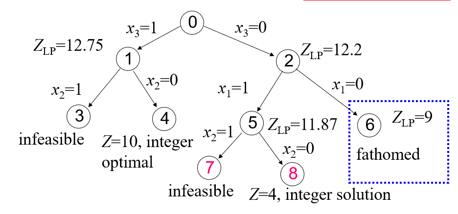
比如:
节点1的partialAssigned == { {x3, 1} }。
节点2的partialAssigned == { {x3, 0} }。
节点3的partialAssigned == { {x3, 1}, {x2, 1} }。
节点4的partialAssigned == { {x3, 1}, {x2, 0} }。
节点7的partialAssigned == { {x3, 0}, {x1, 1}, {x2, 1}}。
然后就可以开始BB过程了:
 public int solveIP() throws IloException {
        while (!this.searchStack.isEmpty()) {
            searchNode branchNode = this.searchStack.pop();
            boolean isVisited = false;
            for (searchNode tempNode: this.visited) {
                if (branchNode.partialAssigned.equals(tempNode.partialAssigned)){
                    isVisited = true;
                    break;
                }
            }

            if (!isVisited) {
                visited.add(new searchNode(branchNode));
                double bound = solveRel.solve(branchNode);
                if (bound > bestVal || bound == 0) {
                    //System.out.println(searchStack.size());
                }
                if (bound < bestVal && bound!=0) {
                    if (branchNode.partialAssigned.size() == solveRel.numTests) {
                        //分支到达低端,找到一个满足整数约束的可行解,设置为当前最优解。
                        //System.out.println("YAY");
                        this.bestVal = bound;
                        this.currentBest = branchNode;
                    }
                }
                if (bound < bestVal && bound!=0) {
                    //如果还没到达低端,找一个变量进行分支。
                    if (branchNode.partialAssigned.size() != solveRel.numTests) {
                        int varToSplit = getSplitVariable(branchNode);
                        if (varToSplit != -1) {
                            searchNode left = new searchNode(branchNode);
                            searchNode right = new searchNode(branchNode);
                            left.partialAssigned.put(varToSplit, 0);
                            right.partialAssigned.put(varToSplit, 1);
                            this.searchStack.push(left);
                            this.searchStack.push(right);
                        }

                    }
                }
            }
        }
        return (int) bestVal;
}首先从搜索栈里面取出一个节点,判断节点代表的分支是否此前已经走过了。
如果没有走过,那么在该节点处进行定界操作,从该节点进入,根据partialAssigned 保存的部分解结构,添加约束,建立松弛模型,调用cplex求解。具体求解过程如下:
public double solve(searchNode node) throws IloException {

      try {
          cplex = new IloCplex();
          cplex.setOut(null);

          IloNumVarType [] switcher = new IloNumVarType[2];
          switcher[0] = IloNumVarType.Int;
          switcher[1] = IloNumVarType.Float;
          int flag = 1;

          IloNumVar[] testUsed = cplex.numVarArray(numTests, 0, 1, switcher[flag]);

          IloNumExpr objectiveFunction = cplex.numExpr();
          objectiveFunction = cplex.scalProd(testUsed, costOfTest);

          cplex.addMinimize(objectiveFunction);

          for (int j = 0; j < numDiseases*numDiseases; j++) {
              if (j % numDiseases == j /numDiseases) {
                  continue;
              }

              IloNumExpr diffConstraint = cplex.numExpr();

              for (int i =  0; i < numTests; i++) {
                  if (A[i][j/numDiseases] == A[i][j%numDiseases]) {
                      continue;
                  }
                  diffConstraint = cplex.sum(diffConstraint, testUsed[i]);
              }

              cplex.addGe(diffConstraint, 1);
              diffConstraint = cplex.numExpr();

          }

          for (int test: node.partialAssigned.keySet()) {
              cplex.addEq(testUsed[test], node.partialAssigned.get(test));
          }


          //System.out.println(cplex.getModel());

          if(cplex.solve()) {
                double objectiveValue = (cplex.getObjValue());

                for (int i = 0; i < numTests; i ++) {
                    if (cplex.getValue(testUsed[i]) == 0) {
                        node.partialAssigned.put(i, 0);
                    }
                    else if (cplex.getValue(testUsed[i]) == 1) {
                        node.partialAssigned.put(i, 1);
                    }
                }
                //System.out.println("LOL"+node.partialAssigned.size());

                return objectiveValue;
          }


      }
      catch(IloException e) {
          System.out.println("Error " + e);
      }
      return 0;
  }
中间一大堆建模过程就不多讲了,具体分支约束是这一句:
for (int test: node.partialAssigned.keySet()) {cplex.addEq(testUsed[test], node.partialAssigned.get(test));}
此后,求解完毕后,把得到整数解的决策变量放进partialAssigned,不是整数后续操作。然后返回目标值。
然后依旧回到solveIP里面,在进行求解以后,得到目标值,接下来就是定界操作了:
if (bound > bestVal || bound == 0):剪支。
if (bound < bestVal && bound!=0):判断是否所有决策变量都为整数,如果是,找到一个可行解,更新当前最优解。如果不是,找一个小数的决策变量入栈,等待后续分支。
运行说明
Example-1:
运行说明,运行输入参数1到3中的数字表示各个不同的模型,需要在32位JDK环境下才能运行,不然会报nullPointer的错误,这是那份求解器wrapper的锅。怎么设置参数参考cplexTSP那篇,怎么设置JDK环境就不多说了。
然后需要把代码文件夹下的几个jar包给添加进去,再把lpsolve的dll给放到native library里面,具体做法还是参照cplexTSP那篇,重复的内容我就不多说了。
Example-2:
最后是运行说明:该实例运行调用了cplex求解器,所以需要配置cplex环境才能运行,具体怎么配置看之前的教程。JDK环境要求64位,无参数输入。
分枝定界算法求解TSP
基本思路
假设有最小化的整数规划问题A,它相应的线性松弛(LP relaxation)规划问题为B。从解问题B开始,若其最优解不符合A的整数条件,那么B的最优目标函数值必是A的最优目标函数值 z* 的下界Z (松弛问题(约束少)最优解 小于等于 原始问题最优解);而 A 的任意可行解的目标函数值将是 z* 的一个上界 z (最优值一定小于等于已经得到的结果)。分枝定界法就是将 A 的可行域分成子区域的方法,逐步增大 Z 和减小z (使非整数解逐渐变为整数解会比当前值Z高,使已经存在的结果接近最优值会降低目标值z),最终求到 z* 。
通常,把全部可行解空间反复地分割为越来越小的子集,称为分枝;并且对每个子集内的解集计算一个目标下界(对于最小值问题),这称为定界。在每次分枝后,凡是界限超出已知可行解集目标值(即上界)的那些子集不再进一步分枝,这样,许多子集可不予考虑,这称为剪枝。
求解TSP通常采用的定界方法是用分配问题定界或者是1-tree来定界。
分配问题的匈牙利算法参考运筹学教学 | 十分钟教你求解分配问题(assignment problem)
关于1-tree我们在这里简单介绍一下,更加详细的介绍将会在之后的附件中给出
在一个图G(V,E)中,节点集合V = {1...n},我们定义{2...n}节点组成的子图的生成树以及两条与1节点的边组成的新图为1-tree。如下图:
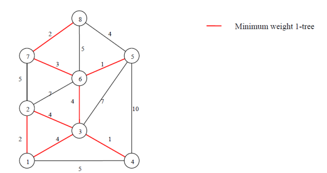
TSP的可行解是1-tree的一种,因此最小权值1-tree (minimum weight 1-tree)可以作为TSP的一个下界,因此可以利用这个性质来作为定界的标准。
最小权值1-tree的很容易求得,只需要求解子图{2...n}的最小生成树再加上两条与1节点相连的最短的边即可。
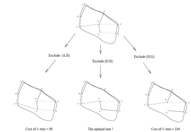
一棵1-tree是一个TSP的可行解的充要条件是1-tree中所有节点的度(degree)均为2。这样分枝的方法也就有了,即寻找1-tree中所有度大于等于3的节点,枚举并依次删除这个节点所有的边,依次求解最小权值1-tree,直到找到可行的TSP解。如下图所示:
整个程序如下所示:
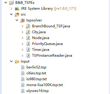
其中各个模块说明如下:
- Timer:计时用。
- TSPInstanceReader:TSPLIB标准算例读取用。
- PriorityQueue:优先队列。
- Node:搜索树的节点。
- City:保存城市的坐标,名字等。
- BranchBound_TSP:BB算法主程序。
branch and bound 过程
搜索树的节点定义,节点定义了原问题的solution和子问题的solution。Node节点定义如下:
public class Node {private ArrayList<Integer> path;private double bound;private int level;public double computeLength(double[][] distanceMatrix) {// TODO Auto-generated method stubdouble distance = 0;for(int i=0;i<this.getPath().size()-1;i++){distance = distance + distanceMatrix[this.getPath().get(i)][this.getPath().get(i+1)];}return distance;}
其余不重要的接口略过。如下:
- path:保存该节点目前已经走过的城市序列。
- bound:记录该节点目前所能达到的最低distance。
- level:记录节点处于搜索树的第几层。
- computeLength:记录当前城市序列的distance。
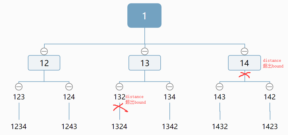
我们知道TSP问题的一个solution是能用一个序列表示城市的先后访问顺序,比如现在有4座城市(1,2,3,4):
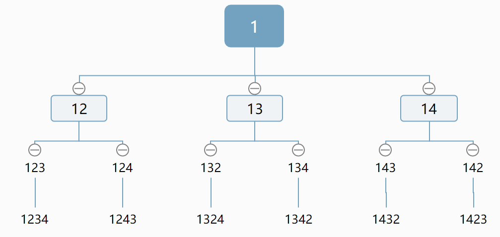
图中每个节点的数字序列就是path保存的。其实分支就是一个穷枚举的过程。
相对于穷举,分支定界算法的优越之处就在于其加入了定界过程,在分支的过程中就砍掉了某些不可能的支,减少了枚举的次数,大大提高了算法的效率。如下:
分支定界算法的主过程如下:
private static void solveTSP(double[][] distanceMatrix) {

        int totalCities = distanceMatrix.length;
        ArrayList<Integer> cities = new ArrayList<Integer>();
        for (int i = 0; i < totalCities; i++) {
            cities.add(i);
        }
        ArrayList<Integer> path;
        double initB = initbound(totalCities, distanceMatrix);

        Node v = new Node(new ArrayList<>(), 0, initB, 0);
        queue.add(v);
        queueCount++;
        while (!queue.isEmpty()) {
            v = queue.remove();
            if (v.getBound() < shortestDistance) {
                Node u = new Node();
                u.setLevel(v.getLevel() + 1);
                for (int i = 1; i < totalCities; i++) {
                    path = v.getPath();
                    if (!path.contains(i)) {
                        u.setPath(v.getPath());
                        path = u.getPath();
                        path.add(i);
                        u.setPath(path);
                        if (u.getLevel() == totalCities - 2) {
                            // put index of only vertex not in u.path at the end
                            // of u.path
                            for (int j = 1; j < cities.size(); j++) {
                                if (!u.getPath().contains(j)) {
                                    ArrayList<Integer> temp = new ArrayList<>();
                                    temp = u.getPath();
                                    temp.add(j);
                                    u.setPath(temp);
                                }
                            }
                            path = u.getPath();
                            path.add(0);
                            u.setPath(path);
                            if (u.computeLength(distanceMatrix) < shortestDistance) {
                                shortestDistance = u.computeLength(distanceMatrix);// implement
                                shortestPath = u.getPath();
                            }
                        } else {
                            u.setBound(computeBound(u, distanceMatrix, cities));
                            //u.getBound()获得的是不完整的解,如果一个不完整的解bound都大于当前最优解,那么完整的解肯定会更大,那就没法玩了。
                            //所以这里只要u.getBound() < shortestDistance的分支
                            if (u.getBound() < shortestDistance) {
                                queue.add(u);
                                queueCount++;
                            }
                            else {
                                System.out.println("currentBest = "+shortestDistance+" cut bound >>> "+u.getBound());
                            }
                        }
                    }
                }
            }
        }
    }
1. 首先initbound利用贪心的方式获得一个bound,作为初始解。
2. 而后利用优先队列遍历搜索树,进行branch and bound算法。对于队列里面的任意一个节点,只有(v.getBound() < shortestDistance)条件成立我们才有分支的必要。不然将该支砍掉。
3. 分支以后判断该支是否到达最底层,这样意味着我们获得了一个完整的解。那么此时就可以更新当前的最优解了。
4. 如果没有到达最底层,则对该支进行定界操作。如果该支的bound也比当前最优解还要大,那么也要砍掉的
然后讲讲定界过程,TSP问题是如何定界的呢?
private static double computeBound(Node u, double[][] distanceMatrix, ArrayList<Integer> cities) {
        double bound = 0;
        ArrayList<Integer> path = u.getPath();
        for (int i = 0; i < path.size() - 1; i++) {
            bound = bound + distanceMatrix[path.get(i)][path.get(i + 1)];
        }
        int last = path.get(path.size() - 1);
        List<Integer> subPath1 = path.subList(1, path.size());
        double min;
        //回来的
        for (int i = 0; i < cities.size(); i++) {
            min = Integer.MAX_VALUE;
            if (!path.contains(cities.get(i))) {
                for (int j = 0; j < cities.size(); j++) {
                    if (i != j && !subPath1.contains(cities.get(j))) {
                        if (min > distanceMatrix[i][j]) {
                            min = distanceMatrix[i][j];
                        }
                    }
                }
            }
            if (min != Integer.MAX_VALUE)
                bound = bound + min;
        }

        //出去的
        min = Integer.MAX_VALUE;
        for (int i = 0; i < cities.size(); i++) {
            if (/*cities.get(i) != last && */!path.contains(i) && min > distanceMatrix[last][i]) {
                min = distanceMatrix[last][i];
            }
        }
        bound = bound + min;
        //System.out.println("bound = "+bound);
        return bound;
}我们知道,每个节点保存的城市序列可能不是完整的解。bound的计算方式:bound = 当前节点path序列的路径距离 + 访问下一个城市的最短路径距离 + 从下一个城市到下下城市(有可能是起点)的最短路径距离。
比如城市节点5个{1,2,3,4,5}。当前path = {1,2},那么:
- 当前节点path序列的路径距离 = d12
- 访问下一个城市的最短路径距离 = min (d2i), i in {3,4,5} (与下一站相关)
- 从下一个城市到下下城市(有可能是起点)的最短路径距离=min (dij), i in {3,4,5} , j in {3,4,5,1}, i != j 。 (与剩余站有关)
注意这两个是可以不相等的。

3、运行说明
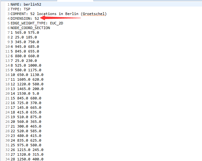
目前分支定界算法解不了大规模的TSP问题,10个节点以内吧差不多。input里面有算例,可以更改里面的DIMENSION值告诉算法需要读入几个节点。
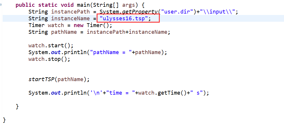
更改算例在main函数下面,改名字就行,记得加上后缀。


 4万+
4万+


 被折叠的 条评论
为什么被折叠?
被折叠的 条评论
为什么被折叠?
 到【灌水乐园】发言


