Pytorch实战语义分割（VOC2012）

本文参照了《动手深度学习》的9.9、9.10章节，原书使用的是 mxnet 框架，本文改成了pytorch代码。
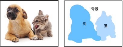
语义分割（semantic segmentation）问题，它关注如何将图像分割成属于不同语义类别的区域。值得一提的是，这些语义区域的标注和预测都是像素级的。

语义分割中图像有关狗、猫和背景的标签

1 图像分割和实例分割

计算机视觉领域还有2个与语义分割相似的重要问题，即图像分割（image segmentation）和实例分割（instance segmentation）：

• 图像分割将图像分割成若干组成区域。这类问题的方法通常利用图像中像素之间的相关性。它在训练时不需要有关图像像素的标签信息，在预测时也无法保证分割出的区域具有我们希望得到的语义。以上图的图像为输入，图像分割可能将狗分割成两个区域：一个覆盖以黑色为主的嘴巴和眼睛，而另一个覆盖以黄色为主的其余部分身体。
• 实例分割又叫同时检测并分割（simultaneous detection and segmentation）。它研究如何识别图像中各个目标实例的像素级区域。与语义分割有所不同，实例分割不仅需要区分语义，还要区分不同的目标实例。如果图像中有两只狗，实例分割需要区分像素属于这两只狗中的哪一只。

2 Pascal VOC2012语义分割数据集

2.1 导入模块

import time
import copy
import torch
from torch import optim, nn
import torch.nn.functional as F
import torchvision
from torchvision import transforms
from torchvision.models import resnet18
import numpy as np
from matplotlib import pyplot as plt
from PIL import Image
import sys
sys.path.append("..")
from IPython import display
from tqdm import tqdm
import warnings
warnings.filterwarnings("ignore") # 忽略警告

2.2 下载数据集

语义分割的一个重要数据集叫作 Pascal VOC2012，点击下载这个数据集的压缩包，大小是 2 GB左右，下载需要一定时间。下载后解压得到 VOCdevkit/VOC2012 文件夹，然后将其放置在 data 文件夹下，VOC2012文件目录是这样的：

• ImageSets/Segmentation 路径包含了指定训练和测试样本的文本文件
• JPEGImages 和 SegmentationClass 路径下分别包含了样本的输入图像和标签。这里的标签也是图像格式，其尺寸和它所标注的输入图像的尺寸相同。标签中颜色相同的像素属于同一个语义类别。

2.3 可视化数据

定义 read_voc_images 函数将输入图像和标签读进内存。

def read_voc_images(root="../../data/VOCdevkit/VOC2012", is_train=True, max_num=None):
    txt_fname = '%s/ImageSets/Segmentation/%s' % (root, 'train.txt' if is_train else 'val.txt')
    with open(txt_fname, 'r') as f:
        images = f.read().split() # 拆分成一个个名字组成list
    if max_num is not None:
        images = images[:min(max_num, len(images))]
    features, labels = [None] * len(images), [None] * len(images)
    for i, fname in tqdm(enumerate(images)):
        # 读入数据并且转为RGB的 PIL image
        features[i] = Image.open('%s/JPEGImages/%s.jpg' % (root, fname)).convert("RGB")
        labels[i] = Image.open('%s/SegmentationClass/%s.png' % (root, fname)).convert("RGB")
    return features, labels # PIL image 0-255

定义可视化数据集的函数 show_images。

# 这个函数可以不需要
def set_figsize(figsize=(3.5, 2.5)):
    """在jupyter使用svg显示"""
    display.set_matplotlib_formats('svg')
    # 设置图的尺寸
    plt.rcParams['figure.figsize'] = figsize

def show_images(imgs, num_rows, num_cols, scale=2):
    # a_img = np.asarray(imgs)
    figsize = (num_cols * scale, num_rows * scale)
    _, axes = plt.subplots(num_rows, num_cols, figsize=figsize)
    for i in range(num_rows):
        for j in range(num_cols):
            axes[i][j].imshow(imgs[i * num_cols + j])
            axes[i][j].axes.get_xaxis().set_visible(False)
            axes[i][j].axes.get_yaxis().set_visible(False)
    plt.show()
    return axes

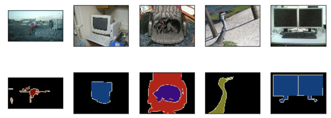
画出前5张输入图像和它们的标签。在标签图像中，白色和黑色分别代表边框和背景，而其他不同的颜色则对应不同的类别。

# 根据自己存放数据集的路径修改voc_dir
voc_dir = r"[local]\VOCdevkit\VOC2012"
train_features, train_labels = read_voc_images(voc_dir, max_num=10)
n = 5 # 展示几张图像
imgs = train_features[0:n] + train_labels[0:n] # PIL image
show_images(imgs, 2, n)

列出标签中每个 RGB 颜色的值及其标注的类别。

# 标签中每个RGB颜色的值
VOC_COLORMAP = [[0, 0, 0], [128, 0, 0], [0, 128, 0], [128, 128, 0],
                [0, 0, 128], [128, 0, 128], [0, 128, 128], [128, 128, 128],
                [64, 0, 0], [192, 0, 0], [64, 128, 0], [192, 128, 0],
                [64, 0, 128], [192, 0, 128], [64, 128, 128], [192, 128, 128],
                [0, 64, 0], [128, 64, 0], [0, 192, 0], [128, 192, 0],
                [0, 64, 128]]
# 标签其标注的类别
VOC_CLASSES = ['background', 'aeroplane', 'bicycle', 'bird', 'boat',
               'bottle', 'bus', 'car', 'cat', 'chair', 'cow',
               'diningtable', 'dog', 'horse', 'motorbike', 'person',
               'potted plant', 'sheep', 'sofa', 'train', 'tv/monitor']

有了上面定义的两个常量以后，我们可以很容易地查找标签中每个像素的类别索引， voc_label_indices 是根据 colormap2label 把标签里的 rgb 颜色对应上面的 VOC_COLORMAP 中的下标给取出来，当作 label 。

colormap2label = torch.zeros(256**3, dtype=torch.uint8) # torch.Size([16777216])
for i, colormap in enumerate(VOC_COLORMAP):
    # 每个通道的进制是256，这样可以保证每个 rgb 对应一个下标 i
    colormap2label[(colormap[0] * 256 + colormap[1]) * 256 + colormap[2]] = i

# 构造标签矩阵
def voc_label_indices(colormap, colormap2label):
    colormap = np.array(colormap.convert("RGB")).astype('int32')
    idx = ((colormap[:, :, 0] * 256 + colormap[:, :, 1]) * 256 + colormap[:, :, 2]) 
    return colormap2label[idx] # colormap 映射 到colormaplabel中计算的下标

可以打印一下结果，这里不展示输出了。

y = voc_label_indices(train_labels[0], colormap2label)
print(y[100:110, 130:140]) #打印结果是一个int型tensor，tensor中的每个元素i表示该像素的类别是VOC_CLASSES[i]

2.4 预处理数据

在语义分割里，如果使用缩放图像使其符合模型的输入形状的话，需要将预测的像素类别重新映射回原始尺寸的输入图像，这样的映射难以做到精确，尤其是在不同语义的分割区域。

所以选择将图像裁剪成固定尺寸而不是缩放。具体来说，我们使用图像增广里的随机裁剪，并对输入图像和标签裁剪相同区域。

def voc_rand_crop(feature, label, height, width):
    """
    随机裁剪feature(PIL image) 和 label(PIL image).
    为了使裁剪的区域相同，不能直接使用RandomCrop，而要像下面这样做
    Get parameters for ``crop`` for a random crop.
    Args:
        img (PIL Image): Image to be cropped.
        output_size (tuple): Expected output size of the crop.
    Returns:
        tuple: params (i, j, h, w) to be passed to ``crop`` for random crop.
    """
    i,j,h,w = torchvision.transforms.RandomCrop.get_params(feature, output_size=(height, width))
    feature = torchvision.transforms.functional.crop(feature, i, j, h, w)
    label = torchvision.transforms.functional.crop(label, i, j, h, w)
    return feature, label

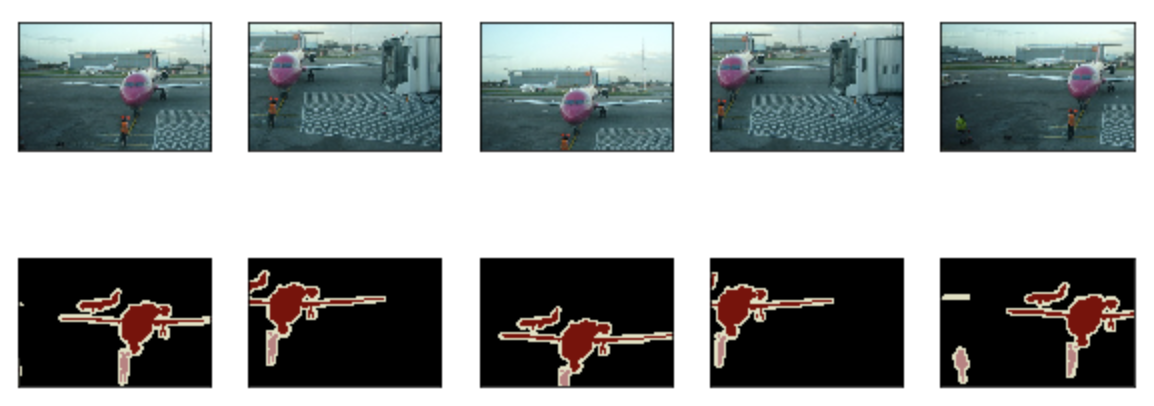
# 显示n张随机裁剪的图像和标签，前面的n是5
imgs = []
for _ in range(n):
    imgs += voc_rand_crop(train_features[0], train_labels[0], 200, 300)
show_images(imgs[::2] + imgs[1::2], 2, n);

3 自定义数据集类

3.1 数据集类

torch.utils.data.Dataset 是表示数据集的抽象类，因此自定义数据集应继承Dataset并覆盖以下方法

• __len__ 实现 len(dataset) 返还数据集的尺寸。
• __getitem__用来获取一些索引数据，例如 dataset[idx] 中的(idx)。

由于数据集中有些图像的尺寸可能小于随机裁剪所指定的输出尺寸，这些样本需要通过自定义的 filter 函数所移除。此外，因为之后会用到预训练模型来做特征提取器，所以我们还对输入图像的 RGB 三个通道的值分别做标准化。

class VOCSegDataset(torch.utils.data.Dataset):
    def __init__(self, is_train, crop_size, voc_dir, colormap2label, max_num=None):
        """
        crop_size: (h, w)
        """
        # 对输入图像的RGB三个通道的值分别做标准化
        self.rgb_mean = np.array([0.485, 0.456, 0.406])
        self.rgb_std = np.array([0.229, 0.224, 0.225])
        self.tsf = torchvision.transforms.Compose([
            torchvision.transforms.ToTensor(),
            torchvision.transforms.Normalize(mean=self.rgb_mean, std=self.rgb_std)])
        self.crop_size = crop_size # (h, w)
        features, labels = read_voc_images(root=voc_dir, is_train=is_train,  max_num=max_num)
# 由于数据集中有些图像的尺寸可能小于随机裁剪所指定的输出尺寸，这些样本需要通过自定义的filter函数所移除
        self.features = self.filter(features) # PIL image
        self.labels = self.filter(labels)     # PIL image
        self.colormap2label = colormap2label
        print('read ' + str(len(self.features)) + ' valid examples')

    def filter(self, imgs):
        return [img for img in imgs if (
            img.size[1] >= self.crop_size[0] and img.size[0] >= self.crop_size[1])]

    def __getitem__(self, idx):
        feature, label = voc_rand_crop(self.features[idx], self.labels[idx], *self.crop_size)
                                # float32 tensor           uint8 tensor (b,h,w)
        return (self.tsf(feature), voc_label_indices(label, self.colormap2label))

    def __len__(self):
        return len(self.features)

3.2 读取数据集

通过自定义的 VOCSegDataset 类来分别创建训练集和测试集的实例。因为待会用的是全卷积网络，所以随机裁剪的输出图像的形状可以自己指定，这里指定为 $320\times 480$。

batch_size = 32 # 实际上我的小笔记本不允许我这么做！哭了（大家根据自己电脑内存改吧）
crop_size = (320, 480) # 指定随机裁剪的输出图像的形状为(320,480)
max_num = 20000 # 最多从本地读多少张图片，我指定的这个尺寸过滤完不合适的图像之后也就只有1175张~

# 创建训练集和测试集的实例
voc_train = VOCSegDataset(True, crop_size, voc_dir, colormap2label, max_num)
voc_test = VOCSegDataset(False, crop_size, voc_dir, colormap2label, max_num)

# 设批量大小为32，分别定义【训练集】和【测试集】的数据迭代器
num_workers = 0 if sys.platform.startswith('win32') else 4
train_iter = torch.utils.data.DataLoader(voc_train, batch_size, shuffle=True,
                              drop_last=True, num_workers=num_workers)
test_iter = torch.utils.data.DataLoader(voc_test, batch_size, drop_last=True,
                             num_workers=num_workers)

# 方便封装，把训练集和验证集保存在dict里
dataloaders = {'train':train_iter, 'val':test_iter}
dataset_sizes = {'train':len(voc_train), 'val':len(voc_test)}

4 构造模型

4.1 预训练模型

下⾯我们使⽤⼀个基于 ImageNet 数据集预训练的 ResNet-18 模型来抽取图像特征。

device = torch.device('cuda' if torch.cuda.is_available() else 'cpu')

num_classes = 21 # 21分类，1个背景，20个物体
model_ft = resnet18(pretrained=True) # 设置True，表明要加载使用训练好的参数

# 特征提取器
for param in model_ft.parameters():
    param.requires_grad = False

4.2 修改成FCN

全卷积⽹络（顾名思义就是全部都是卷积层）先使⽤卷积神经⽹络抽取图像特征，然后通过 $1\times 1$ 卷积层将通道数变换为类别个数（21类），最后通过转置卷积层将特征图的⾼和宽变换为输⼊图像的尺⼨。模型输出与输⼊图像的⾼和宽要相同，并在空间位置上（像素级）⼀⼀对应，则最终输出的 tensor 在通道方向包含了该空间位置像素的类别预测（每个像素对应 21 个通道，数值对应21个类别的probability）。

可以先打印 model_ft 查看网络结构，可知 ResNet-18 的最后两层分别是全局最⼤池化层GlobalAvgPool2D 和 全连接层，而 FCN 不需要这些层，所以我们要把这两层去掉。

通过测试，当输入图像的 size 是$(batch,3,320,480)$ 时，经过除最后两层的预训练网络的输出的大小是 $(batch,512,10,15)$，也就是 $feature$ 的宽高比输入缩小了 $32$ 倍，那么只需要用转置卷积层将其放大 $32$ 倍即可。

其中，对于转置卷积层，如果步幅为 $S$、填充为 $S/2$ （假设为整数）、卷积核的⾼和宽为 $2S$，转置卷积核将输⼊的⾼和宽分别放⼤ $S$ 倍。这样就得到了转置卷积层的参数nn.ConvTranspose2d(num_classes,num_classes, kernel_size=64, padding=16, stride=32).

model_ft = nn.Sequential(*list(model_ft.children())[:-2], # 去掉最后两层
              nn.Conv2d(512,num_classes,kernel_size=1), # 用大小为1的卷积层改变输出通道为num_class
              nn.ConvTranspose2d(num_classes,num_classes, kernel_size=64, padding=16, stride=32)).to(device) # 转置卷积层使图像变为输入图像的大小

# 对model_ft做一个测试
x = torch.rand((2,3,320,480), device=device) # 构造随机的输入数据
print(net(x).shape) # 输出依然是 torch.Size([2, 21, 320, 480]) 

# 打印第一个小批量的类型和形状。不同于图像分类和目标识别，这里的标签是一个三维数组
# for X, Y in train_iter:
#     print(X.dtype, X.shape)
#     print(Y.dtype, Y.shape)
#     break

4.3 初始化转置卷积层

在图像处理中，我们有时需要将图像放⼤，即上采样（upsample）。上采样的⽅法有很多，常⽤的有双线性插值。简单来说，为了得到输出图像

在坐标 $(x,y)$上的像素，先将该坐标映射到输⼊图像的坐标 $(x\prime ,y\prime )$。例如，根据输⼊与输出的尺⼨之⽐来映射。映射后的 $x\prime$ 和 $y\prime$ 通常是实数。然后，在输⼊图像上找到与坐标 $(x\prime ,y\prime )$最近的 $4$ 个像素。最后，输出图像在坐标 $(x,y)$上的像素依据输⼊图像上这$4$个像素及其与 $(x\prime ,y\prime )$的相对距离来计算。双线性插值的上采样可以通过由以下 bilinear_kernel 函数构造的卷积核的转置卷积层来实现。

# 双线性插值的上采样，用来初始化转置卷积层的卷积核
def bilinear_kernel(in_channels, out_channels, kernel_size):
    factor = (kernel_size+1)//2
    if kernel_size%2 == 1:
        center = factor-1
    else:
        center = factor-0.5
    og = np.ogrid[:kernel_size, :kernel_size]
    filt = (1-abs(og[0]-center)/factor) * (1-abs(og[1]-center)/factor)
    weight = np.zeros((in_channels,out_channels, kernel_size,kernel_size), dtype='float32')
    weight[range(in_channels), range(out_channels), :, :] = filt
    weight = torch.Tensor(weight)
    weight.requires_grad = True
    return weight

在全卷积⽹络中，将转置卷积层初始化为双线性插值的上采样。对于$1\times 1$卷积层，采⽤ $Xavier$ 随机初始化。

nn.init.xavier_normal_(model_ft[-2].weight.data, gain=1)
model_ft[-1].weight.data = bilinear_kernel(num_classes, num_classes, 64).to(device)

5 训练模型

现在可以开始训练模型了。这⾥的损失函数和准确率计算与图像分类中的并没有本质上的不同，即是在通道方向上计算 交叉熵误差 。有一个 blog 我认为说的很详细，图也画得很好：https://blog.csdn.net/Fcc_bd_stars/article/details/105158215

def train_model(model:nn.Module, criterion, optimizer, scheduler, num_epochs=20):
    since = time.time()
    best_model_wts = copy.deepcopy(model.state_dict())
    best_acc = 0.0
    # 每个epoch都有一个训练和验证阶段
    for epoch in range(num_epochs):
        print('Epoch {}/{}'.format(epoch, num_epochs-1))
        print('-'*10)
        for phase in ['train', 'val']:
            if phase == 'train':
                scheduler.step()
                model.train()
            else:
                model.eval()
            runing_loss = 0.0
            runing_corrects = 0.0
            # 迭代一个epoch
            for inputs, labels in dataloaders[phase]:
                inputs, labels = inputs.to(device), labels.to(device)
                optimizer.zero_grad() # 零参数梯度
				# 前向，只在训练时跟踪参数
                with torch.set_grad_enabled(phase=='train'):
                    logits = model(inputs)  # [5, 21, 320, 480]
                    loss = criteon(logits, labels.long())
                    # 后向，只在训练阶段进行优化
                    if phase=='train':
                        loss.backward()
                        optimizer.step()
				# 统计loss和correct
                runing_loss += loss.item()*inputs.size(0)
                runing_corrects += torch.sum((torch.argmax(logits.data,1))==labels.data)/(480*320)

            epoch_loss = runing_loss / dataset_sizes[phase]
            epoch_acc = runing_corrects.double() / dataset_sizes[phase]
            print('{} Loss: {:.4f} Acc: {:.4f}'.format(phase, epoch_loss, epoch_acc))
			# 深度复制model参数
            if phase=='val' and epoch_acc>best_acc:
                best_acc = epoch_acc
                best_model_wts = copy.deepcopy(model.state_dict())
        print()
    time_elapsed = time.time() - since;
    print('Training complete in {:.0f}m {:.0f}s'.format(time_elapsed//60, time_elapsed%60))
    # 加载最佳模型权重
    model.load_state_dict(best_model_wts)
    return model

下面定义train_model要用到的参数，开始训练

epochs = 5 # 训练5个epoch
criteon = nn.CrossEntropyLoss()
optimizer = optim.SGD(model_ft.parameters(), lr=0.001, weight_decay=1e-4, momentum=0.9)
# 每3个epochs衰减LR通过设置gamma=0.1
exp_lr_scheduler = optim.lr_scheduler.StepLR(optimizer, step_size=3, gamma=0.1)

# 开始训练
model_ft = train_model(model_ft, criteon, optimizer, exp_lr_scheduler, num_epochs=epochs)

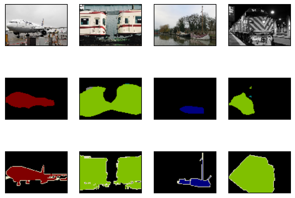
6 测试模型

为了可视化每个像素的预测类别，我们将预测类别映射回它们在数据集中的标注颜⾊。

def label2image(pred):
    # pred: [320,480]
    colormap = torch.tensor(VOC_COLORMAP,device=device,dtype=int)
    x = pred.long()
    return (colormap[x,:]).data.cpu().numpy()

下面这里提供了两种测试形式

6.1 通用型

其实如果要用于测试其它数据集，也是要改动一下的 : ) 😃

mean=torch.tensor([0.485, 0.456, 0.406]).reshape(3,1,1).to(device)
std=torch.tensor([0.229, 0.224, 0.225]).reshape(3,1,1).to(device)
def visualize_model(model:nn.Module, num_images=4):
    was_training = model.training
    model.eval()
    images_so_far = 0
    n, imgs = num_images, []
    with torch.no_grad():
        for i, (inputs, labels) in enumerate(dataloaders['val']):
            inputs, labels = inputs.to(device), labels.to(device) # [b,3,320,480]
            outputs = model(inputs)
            pred = torch.argmax(outputs, dim=1) # [b,320,480]
            inputs_nd = (inputs*std+mean).permute(0,2,3,1)*255 # 记得要变回去哦

            for j in range(num_images):
                images_so_far += 1
                pred1 = label2image(pred[j]) # numpy.ndarray (320, 480, 3)
                imgs += [inputs_nd[j].data.int().cpu().numpy(), pred1, label2image(labels[j])]
                if images_so_far == num_images:
                    model.train(mode=was_training)
                    # 我已经固定了每次只显示4张图了，大家可以自己修改
                    show_images(imgs[::3] + imgs[1::3] + imgs[2::3], 3, n)
                    return model.train(mode=was_training)

# 开始验证
visualize_model(model_ft)

6.2 不通用

在预测时，我们需要将输⼊图像在各个通道做标准化，并转成卷积神经⽹络所需要的四维输⼊格式。

# 预测前将图像标准化，并转换成(b,c,h,w)的tensor
def predict(img, model):
    tsf = transforms.Compose([
            transforms.ToTensor(), # 好像会自动转换channel
            transforms.Normalize(mean=[0.485, 0.456, 0.406], std=[0.229, 0.224, 0.225])])
    x = tsf(img).unsqueeze(0).to(device) # (3,320,480) -> (1,3,320,480)
    pred = torch.argmax(model(x), dim=1) # 每个通道选择概率最大的那个像素点 -> (1,320,480)
    return pred.reshape(pred.shape[1],pred.shape[2]) # reshape成(320,480)

def evaluate(model:nn.Module):
    model.eval()
    test_images, test_labels = read_voc_images(voc_dir, is_train=False, max_num=10) 
    n, imgs = 4, []
    for i in range(n):
        xi, yi = voc_rand_crop(test_images[i], test_labels[i], 320, 480) # Image
        pred = label2image(predict(xi, model))
        imgs += [xi, pred, yi]
    show_images(imgs[::3] + imgs[1::3] + imgs[2::3], 3, n)

# 开始测试
evaluate(model_ft)

7 结语

训练了3个epoch我的输出：

Epoch 0/2
----------
train Loss: 1.7844 Acc: 0.5835
val Loss: 1.1669 Acc: 0.6456

Epoch 1/2
----------
train Loss: 1.1288 Acc: 0.6535
val Loss: 0.9012 Acc: 0.6929

Epoch 2/2
----------
train Loss: 0.8578 Acc: 0.6906
val Loss: 0.7988 Acc: 0.7568

Training complete in 6m 37s

可以看见训练时间不需要很长，我试过 epochs = 5 时，训练集的精度在 $89$% 左右，测试集的精度可以达到 $86$ %。

对于这个模型用 ResNet-50 作特征提取器会有更好的效果，不过训练的时间也会更长。还有超参数lr, weight_decay, momentum, step_size, gamma 以及$1\times 1$卷积层和转置卷积层的初始化方式也可以继续调。

语义分割还有很多可用的模型，本文用的是 FCN，在其它一些模型上会有更好的表现：

• Deeplab V3+ 具有可分离卷积的编码器/解码器，用于语义图像分割
• GCN 通过全局卷积网络改进语义分割
• UperNet 统一感知解析
• ENet 用于实时语义分割的深度神经网络体系结构
• U-Net 用于生物医学图像分割的卷积网络
• SegNet 用于图像分段的深度卷积编码器-解码器架构。
  还有（DUC，HDC）、PSPNet等。

常用的语义分割数据集也有很多：Pascal VOC、CityScapes、ADE20K、COCO Stuff等。

对于损失函数，除了交叉熵误差，也可以用这些：

• Dice-Loss 可以测试两个样本之间的重叠度量，可以更好地反映训练目标，但该损失函数具有很强的非凸性，很难优化。
• CE Dice loss Dice 损失与 CE 的总和，CE 提供了平滑的优化，而 Dice 损失则很好地表明了分割结果的质量。
• Focal Loss CE 的另一种版本，用于避免类别不平衡而降低了置信度的情况。
• Lovasz Softmax 查看论文：Lovasz - softmax损失。