人群计数：Rethinking Counting and Localization in Crowds: A Purely Point-Based Framework

学习链接：ICCV 2021 Oral | 重新思考人群计数和定位：一个纯粹基于点的框架
学习链接：论文解读Rethinking Counting and Localization in Crowds: A Purely Point-Based Framework
FPN网络详解：FPN网络详解

P2PNet论文：

解决的问题：

• 在人群中定位个体更符合后续高级人群分析任务的实际需求，而不是简单地计数。然而，现有的基于定位的方法依赖于作为学习目标的中间表示（即密度图或伪框）是违反直觉和容易出错的。
• 现有的评价指标没有很好的兼顾计数和定位两方面的评价。现有的对定位感知指标要么忽略了人群中的显著密度变化，要么缺乏对重复预测的惩罚。

解决方案：提出了一个纯粹的基于点的框架，用于在人群中进行实现计数和个体定位。

文章贡献：

• 提出了一个纯粹的基于点的框架，用于在人群中进行实现计数和个体定位；
• 提出了密度归一化平均精度(density Normalized Average Precision)作为新框架下的综合评价指标，以兼顾定位和计数两方面的评价；
• 提出P2PNet网络结构作为一种直观的解决方案，遵循这个概念上实现简单的框架。该方法实现了最先进的计数精度和有前景的本地化性能，并可能为其他依赖点预测的任务提供启发。

前言

其他方法的一些缺点，自身方法的优点：
且基于检测框的方法标注费力。

纯基于点的框架

提出的框架直接以点标注作为学习目标，然后提供人群中每个人的确切位置，不止是简单的计数。

对该框架的详细介绍：
给定一张带有N个人的图像，每个人头中心点用一个坐标$(x_i,y_i)$表示，对应集合则为$P_N$。网络输出两个东西，一个是预测头部的中心点$P_M^{{}^{\prime }}$，一个是该中心点的置信度$C$。目标是使预测点与ground truth尽可能地接近，并有足够高的置信度。

与传统的计数方法相比，该框架提供的个体位置有助于那些基于运动的人群分析任务，如人群跟踪、活动识别、异常检测等 此外，该框架不依赖于劳动密集型标注、不准确的伪框或棘手的后处理，受益于原始点表示的高精度定位特性，特别是对于人群中高度拥挤的区域。

密度归一化平均精度

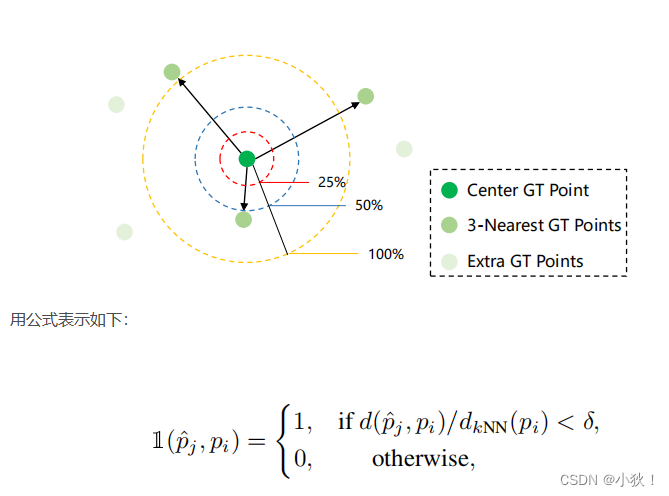
一个预测点$p_j$只有在它可以匹配到某个真值点$p_i$时才被归类为$TP$，且这个真值点之前没有被得分更高的预测点匹配上，匹配过程用像素级的欧几里得距离来指导。【然而】如果直接使用像素距离来测量亲和度忽略了人群之间大密度变化的副作用，为此匹配标准引入了密度归一化，以缓解密度变化问题。（也就是一个好的参考点可能与多个真值点进行匹配，但最终只能一对一匹配，这样计数就可能变少了，尤其是在密度大的时候。也就是之前匹配过的没有给排斥掉）

也就是引入最近邻$k$（取3）个点，将它们的距离归一化。
黄圈是$d_{kNN}(p_i)$的中心真值点$p_i$点像素的距离，蓝圈一半，红圈1/4。假设参数值$\delta$为0.5，也就是蓝圈，那么在这个区域里面就把中心点$p_i$当作真值点，对应的，红圈的话，也就代表着更严格的定位准确率。

匈牙利算法点匹配方法

匈牙利算法讲解学习链接：算法学习笔记(5)：匈牙利算法
总体问题：也就是说如何实现真值点和预测点的一一对应问题。

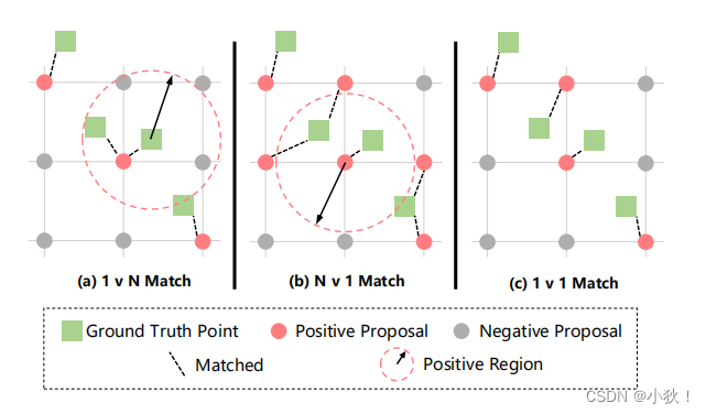
训练阶段采用一种相互最优的一对一匹配策略。对于每个真值点，选择距离最近的参考点应该产生最好的预测结果。
然而，如果我们为每个真值点选择最近的参考点，很可能一个参考点与多个匹配，如图(a)所示，在这种情况下，只有一个真值点匹配到参考点，这样会导致低估的计数，特别是在人群拥挤的区域。
其次，对于每个参考点，我们可以将最近的真值点指定为匹配目标，虽然这种策略可能有助于减轻优化的总体开销，但是还是可能会有多个参考点与同一个真值点匹配，如图(b)所示。这可能会导致高估计数。

因此，关联过程通常要考虑到双方的情况，产生相互最优的一对一匹配结果，如图©所示。（也即使用匈牙利算法。）

此外，其他两种策略都必须确定一个阈值，而与其匹配目标的距离超过这个阈值的参考点将被视为Negative Proposal。在一对一匹配时，那些未匹配的建议将自动保留为背景点，积极的参考点应被推向其目标，由于参考点的位置是随着训练过程动态更新的，那些有潜力表现更好的参考点可以通过一对一匹配逐渐选择作为最终预测。

P2PNet

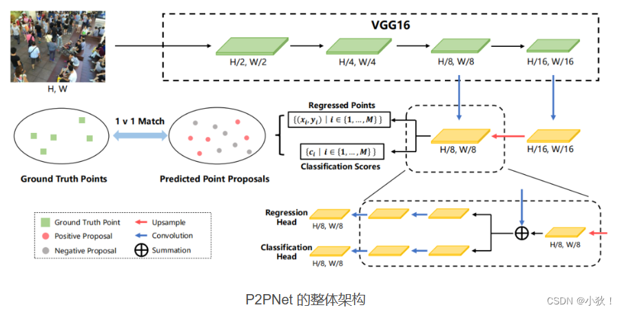
P2PNet的主干网络为VGG16，VGG16第四个阶段输出上采样后与第三阶段输出特征图进行融合。融合之后，分别进行头部位置回归以及置信度计算。两个分支分别经过三个卷积，得到H/8,W/8大小的特征图。

代码中实现过程如下：
输入网络的大小为[32,3,128,128]
经过VGG16的四个body后，大小分别为
[32,128,64,64]->[32,256,32,32](C3)->[32,512,16,16](C4)->[32,512,8,8](C5)
将后一层上采样与当前层相加。
P5_x是经过C5自身的P5_1之后上采样，然后经过P5_2得到最终的P5_x[32,256,8,8].
C5上采样与经过P4_1的C4进行像素级相加得到P4_x，再经过P4_2，得到最终的P4_x[32,256,16,16]。
P4_x上采样与经过P3_1的C3进行像素级相加得到P3_x，再经过P3_2，得到最终的P3_x[32,256,32,32]（没用）。

代码中后面两个分别计算头部位置回归偏移量[32,1024,2]（偏移量+anchor点位置）和置信度[32,1024,2]的两个分支网络（分别由三个卷积层组成），均使用P4_x作为输入进行最终的计算。

regression分支：[32,256,16,16]->[32,256,16,16]->[32,8,16,16]
然后使用permute(0,2,3,1)函数使之成为[32,16,16,8]，然后使用contiguous().view(out.shape[0], -1, 2)使之成为[32,1024,2]，因此这个2是从通道数8里面分出来的。

classification分支：[32,256,16,16]->[32,256,16,16]->[32,8,16,16]然后使用permute(0,2,3,1)函数使之成为[32,16,16,8]。因为有两类，所以num.classes是2，anchor_points对应为4，使用下面这两个函数使之转为[32,1024,2]大小的变量，与前面regression大小对应。

batch_size, width, height, _ = out1.shape # 32, 16, 16, 8
out2 = out1.view(batch_size, width, height, self.num_anchor_points, self.num_classes) # [32,16,16,4,2]

anchorpoints点设置：网格状的位置覆盖整个图片，stride步幅用了8，anchor点的生成过程可以看下面代码。[1,1024,2]，32个batch则变成了[32,1024,2]。其中anchor小矩阵与基础点的相加使用了广播机制。
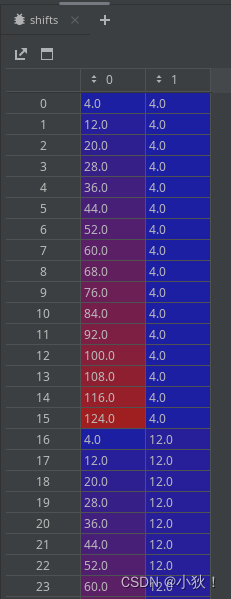
假设图片大小为128*128，步幅为8，那么得出的图片基础点的矩阵为[16,16]，也就是行列的[ 4. 12. 20. 28. 36. 44. 52. 60. 68. 76. 84. 92. 100. 108., 116. 124.]。
详细解释：

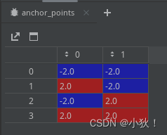
1. 首先利用步幅计算得出小范围的meshgrid网格anchor_points[4,2]，如下图：代表着在基础点的基础上对其作这个小网格的运算，详见后续。
   

2. 用[16，]的x,y两组基础点坐标绘制[16,16]的网格，而后利用np.vstack函数对其进行组合成[256,2]的坐标点。部分如下图
   

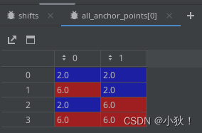
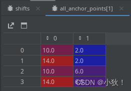
3. 利用reshape和transpose函数，将1和2中得到的数组转为[1,4,2]和[256,1,2]大小的数组，利用广播机制进行相加（也就是2中的第一行与1的每一行进行相加得到[4,2]，2的第二行也与1的每一行相加得到[4,2]，对应意义为在基础点的基础上网格状周围几个点），得到[256,4,2]的all_anchor_points数组，它的第一个，第二个元素值为：
   

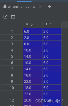
4. 最后将其转为[1024,2]大小数组，对应一幅图中1024个坐标点。
   

P2PNet网络代码：

class P2PNet(nn.Module):
    def __init__(self, backbone, row=2, line=2):
        super().__init__()
        self.backbone = backbone
        self.num_classes = 2
        # the number of all anchor points
        num_anchor_points = row * line

        self.regression = RegressionModel(num_features_in=256, num_anchor_points=num_anchor_points)
        self.classification = ClassificationModel(num_features_in=256, \
                                            num_classes=self.num_classes, \
                                            num_anchor_points=num_anchor_points)

        self.anchor_points = AnchorPoints(pyramid_levels=[3,], row=row, line=line) # stride:[8]

        self.fpn = Decoder(256, 512, 512) #FPN层

    def forward(self, samples: NestedTensor):
        # get the backbone features
        features = self.backbone(samples)
        # forward the feature pyramid
        features_fpn = self.fpn([features[1], features[2], features[3]])

        batch_size = features[0].shape[0] # 32
        # run the regression and classification branch
        regression = self.regression(features_fpn[1]) * 100 # 8x  # [32,1024,2]
        classification = self.classification(features_fpn[1]) # [32,1024,2]
        anchor_points = self.anchor_points(samples).repeat(batch_size, 1, 1) # [32,1024,2]
        # decode the points as prediction
        output_coord = regression + anchor_points # 预测的点的位置+偏移量 # [32,1024,2]
        output_class = classification # 置信度 # [32,1024,2]
        out = {'pred_logits': output_class, 'pred_points': output_coord}
       
        return out

FPN层的代码：

class Decoder(nn.Module):
    def __init__(self, C3_size, C4_size, C5_size, feature_size=256):
        super(Decoder, self).__init__()

        # upsample C5 to get P5 from the FPN paper
        self.P5_1 = nn.Conv2d(C5_size, feature_size, kernel_size=1, stride=1, padding=0)
        self.P5_upsampled = nn.Upsample(scale_factor=2, mode='nearest')
        self.P5_2 = nn.Conv2d(feature_size, feature_size, kernel_size=3, stride=1, padding=1)

        # add P5 elementwise to C4
        self.P4_1 = nn.Conv2d(C4_size, feature_size, kernel_size=1, stride=1, padding=0)
        self.P4_upsampled = nn.Upsample(scale_factor=2, mode='nearest')
        self.P4_2 = nn.Conv2d(feature_size, feature_size, kernel_size=3, stride=1, padding=1)

        # add P4 elementwise to C3
        self.P3_1 = nn.Conv2d(C3_size, feature_size, kernel_size=1, stride=1, padding=0)
        self.P3_upsampled = nn.Upsample(scale_factor=2, mode='nearest')
        self.P3_2 = nn.Conv2d(feature_size, feature_size, kernel_size=3, stride=1, padding=1)


    def forward(self, inputs):
        C3, C4, C5 = inputs # C3:[32,256,32,32],C4:[32,512,16,16],C5:[32,512,8,8]

        P5_x = self.P5_1(C5) # [32,256,8,8]
        P5_upsampled_x = self.P5_upsampled(P5_x) # [32,256,16,16]
        P5_x = self.P5_2(P5_x) # [32,256,8,8]

        P4_x = self.P4_1(C4) # [32,256,16,16]
        P4_x = P5_upsampled_x + P4_x # [32,256,16,16] 元素级相加
        P4_upsampled_x = self.P4_upsampled(P4_x) # [32,256,32,32]
        P4_x = self.P4_2(P4_x)# [32,256,16,16]

        P3_x = self.P3_1(C3)# [32,256,16,16]
        P3_x = P3_x + P4_upsampled_x # [32,256,32,32]
        P3_x = self.P3_2(P3_x) # [32,256,32,32]

        return [P3_x, P4_x, P5_x]

RegressionModel代码：

class RegressionModel(nn.Module):
    def __init__(self, num_features_in, num_anchor_points=4, feature_size=256):
        super(RegressionModel, self).__init__()

        self.conv1 = nn.Conv2d(num_features_in, feature_size, kernel_size=3, padding=1)
        self.act1 = nn.ReLU()

        self.conv2 = nn.Conv2d(feature_size, feature_size, kernel_size=3, padding=1)
        self.act2 = nn.ReLU()

        self.conv3 = nn.Conv2d(feature_size, feature_size, kernel_size=3, padding=1)
        self.act3 = nn.ReLU()

        self.conv4 = nn.Conv2d(feature_size, feature_size, kernel_size=3, padding=1)
        self.act4 = nn.ReLU()

        self.output = nn.Conv2d(feature_size, num_anchor_points * 2, kernel_size=3, padding=1)
    # sub-branch forward
    def forward(self, x):  # [32,256,16,16]
        out = self.conv1(x) # [32,256,16,16]
        out = self.act1(out) # [32,256,16,16]

        out = self.conv2(out) # [32,256,16,16]
        out = self.act2(out) # [32,256,16,16]

        out = self.output(out) # [32,8,16,16]

        out = out.permute(0, 2, 3, 1) # [32,16,16,8]

        return out.contiguous().view(out.shape[0], -1, 2) #[32,1024,2]

classification分支代码：

# the network frmawork of the classification branch
class ClassificationModel(nn.Module):
    def __init__(self, num_features_in, num_anchor_points=4, num_classes=80, prior=0.01, feature_size=256):
        super(ClassificationModel, self).__init__()

        self.num_classes = num_classes # 2
        self.num_anchor_points = num_anchor_points

        self.conv1 = nn.Conv2d(num_features_in, feature_size, kernel_size=3, padding=1)
        self.act1 = nn.ReLU()

        self.conv2 = nn.Conv2d(feature_size, feature_size, kernel_size=3, padding=1)
        self.act2 = nn.ReLU()

        self.conv3 = nn.Conv2d(feature_size, feature_size, kernel_size=3, padding=1)
        self.act3 = nn.ReLU()

        self.conv4 = nn.Conv2d(feature_size, feature_size, kernel_size=3, padding=1)
        self.act4 = nn.ReLU()

        self.output = nn.Conv2d(feature_size, num_anchor_points * num_classes, kernel_size=3, padding=1)
        self.output_act = nn.Sigmoid()
    # sub-branch forward
    def forward(self, x):
        out = self.conv1(x)
        out = self.act1(out)

        out = self.conv2(out)
        out = self.act2(out)

        out = self.output(out) # [32,8,16,16]

        out1 = out.permute(0, 2, 3, 1) # [32,16,16,8]

        batch_size, width, height, _ = out1.shape # 32, 16, 16, 8

        out2 = out1.view(batch_size, width, height, self.num_anchor_points, self.num_classes) # [32,16,16,4,2]

        return out2.contiguous().view(x.shape[0], -1,  self.num_classes) #[32,1024,2]

生成anchor_points的代码：

# generate the reference points in grid layout
def generate_anchor_points(stride=16, row=3, line=3): # 8,2,2
    row_step = stride / row  # 4
    line_step = stride / line # 4

    shift_x = (np.arange(1, line + 1) - 0.5) * line_step - stride / 2 # [-2,2]
    shift_y = (np.arange(1, row + 1) - 0.5) * row_step - stride / 2 # [-2,2]

    shift_x, shift_y = np.meshgrid(shift_x, shift_y) # shift_x:[[-2.  2.], [-2.  2.]],shift_y:[[-2. -2.], [ 2.  2.]]

    anchor_points = np.vstack(( # 按垂直方向（行顺序）堆叠数组构成一个新的数组,堆叠的数组需要具有相同的维度
        shift_x.ravel(), shift_y.ravel() # ravel函数的功能是将原数组拉伸成为一维数组
    )).transpose() # transpose()函数的作用就是调换数组的行列值的索引值，类似于求矩阵的转置

    return anchor_points # [[-2. -2.], [ 2. -2.], [-2.  2.], [ 2.  2.]]

# shift the meta-anchor to get an acnhor points
def shift(shape, stride, anchor_points):
    shift_x = (np.arange(0, shape[1]) + 0.5) * stride # [  4.  12.  20.  28.  36.  44.  52.  60.  68.  76.  84.  92. 100. 108., 116. 124.]
    shift_y = (np.arange(0, shape[0]) + 0.5) * stride

    shift_x, shift_y = np.meshgrid(shift_x, shift_y) #

    shifts = np.vstack((
        shift_x.ravel(), shift_y.ravel()
    )).transpose() # [256,2]

    A = anchor_points.shape[0] # 4
    K = shifts.shape[0] # 256
    all_anchor_points = (anchor_points.reshape((1, A, 2)) + shifts.reshape((1, K, 2)).transpose((1, 0, 2))) #[256,4,2]，广播机制
    all_anchor_points = all_anchor_points.reshape((K * A, 2)) # [1024,2]

    return all_anchor_points

# this class generate all reference points on all pyramid levels
class AnchorPoints(nn.Module):
    def __init__(self, pyramid_levels=None, strides=None, row=3, line=3):
        super(AnchorPoints, self).__init__()

        if pyramid_levels is None:
            self.pyramid_levels = [3, 4, 5, 6, 7]
        else:
            self.pyramid_levels = pyramid_levels # pyramid_levels: [3]

        if strides is None:
            self.strides = [2 ** x for x in self.pyramid_levels] # [8]

        self.row = row # 2
        self.line = line # 2

    def forward(self, image):
        image_shape = image.shape[2:] #[128,128]图像大小 [32,3,128,128]
        image_shape = np.array(image_shape) #[128,128]
        image_shapes = [(image_shape + 2 ** x - 1) // (2 ** x) for x in self.pyramid_levels] # [16,16], x=3

        all_anchor_points = np.zeros((0, 2)).astype(np.float32)
        # get reference points for each level
        for idx, p in enumerate(self.pyramid_levels):
            anchor_points = generate_anchor_points(2**p, row=self.row, line=self.line) #[4,2]
            shifted_anchor_points = shift(image_shapes[idx], self.strides[idx], anchor_points) # [1024,2]
            all_anchor_points = np.append(all_anchor_points, shifted_anchor_points, axis=0) # [1024,2]

        all_anchor_points = np.expand_dims(all_anchor_points, axis=0) #[1,1024,2]
        # send reference points to device
        if torch.cuda.is_available():
            return torch.from_numpy(all_anchor_points.astype(np.float32)).cuda()
        else:
            return torch.from_numpy(all_anchor_points.astype(np.float32))

测试部分代码（下）：利用0.5大小的阈值，进行softmax操作之后大于0.5的保留这个人头。

 # run inference
    outputs = model(samples)
    outputs_scores = torch.nn.functional.softmax(outputs['pred_logits'], -1)[:, :, 1][0]

    outputs_points = outputs['pred_points'][0]

    threshold = 0.5
    # filter the predictions
    points = outputs_points[outputs_scores > threshold].detach().cpu().numpy().tolist()
    predict_cnt = int((outputs_scores > threshold).sum())

P2PNet的代码中使用了FPN层。
FPN层详解链接：CSDN-FPN网络详解

横向链接：

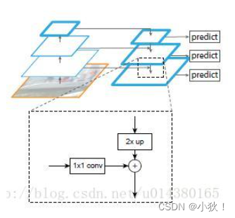
①自底向上：

自底向上的过程就是神经网络普通的前向传播过程，特征图经过卷积核计算，通常会越变越小。

具体而言，对于ResNets，我们使用每个阶段的最后一个residual block输出的特征激活输出。对于conv2，conv3，conv4和conv5输出，我们将这些最后residual block的输出表示为{C2，C3，C4，C5}，并且它们相对于输入图像具有{4, 8, 16, 32} 的步长。由于其庞大的内存占用，我们不会将conv1纳入金字塔中。

②自上而下：
自上而下的过程是把更抽象、语义更强的高层特征图进行上采样（upsampling），而横向连接则是将上采样的结果和自底向上生成的相同大小的feature map进行融合（merge）。横向连接的两层特征在空间尺寸相同，这样做可以利用底层定位细节信息。将低分辨率的特征图做2倍上采样（为了简单起见，使用最近邻上采样）。然后通过按元素相加，将上采样映射与相应的自底而上映射合并。这个过程是迭代的，直到生成最终的分辨率图。
为了开始迭代，我们只需在C5上附加一个1×1卷积层来生成低分辨率图P5。最后，我们在每个合并的图上附加一个3×3卷积来生成最终的特征映射，这是为了减少上采样的混叠效应。这个最终的特征映射集称为{P2，P3，P4，P5}，分别对应于{C2，C3，C4，C5}，它们具有相同的尺寸。
由于金字塔的所有层次都像传统的特征化图像金字塔一样使用共享分类器/回归器，因此我们在所有特征图中固定特征维度（通道数，记为d）。

③横向连接：
采用1×1的卷积核进行连接（减少特征图数量）。

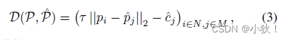
匹配部分

点匹配使用了匈牙利算法，D是真值点和预测点之间的代价矩阵，定义如下，其中$c$是预测点对应的置信度，基于此矩阵利用匈牙利算法进行匹配：

损失函数：

上面类别置信度计算利用交叉熵损失函数，下面点位置损失使用欧几里得距离进行计算。

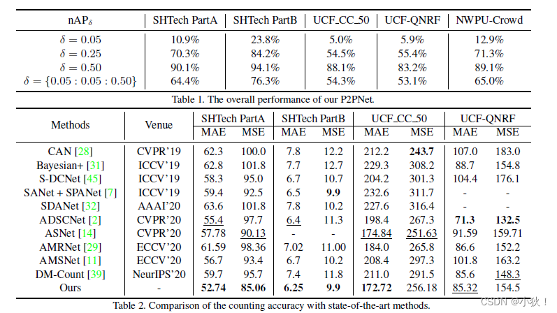
实验

数据集：ShanghaiTech PartA and PartB, UCF CC 50（five-fold cross validation）, UCF-QNRFand NWPU-Crowd.
对应结果：

消融实验

1. 像素参考点的位置，是网格还是中心点，也就是anchor点，实验证明两者都挺好，但网格表现更好，因为密度更大。
   
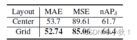
2. P2PNet的步幅
   
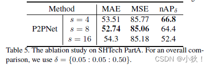
   这三个效果都很好，说明基于点的方法的有效性。步幅为8的时候的效果最好。步幅为6的时候nAP结果更好得出：更精细的特征图更利于定位。