论文学习--Multi-View Attribute Graph Convolution Networks for Clustering(MAGCN)

一、论文题目

Multi-View Attribute Graph Convolution Networks for Clustering

二、Abstract

（一）本文提出的问题

1.在GNN中，现有方法无法将可学习的权重分配给邻域中的不同节点，并且由于忽略节点属性和图重建而缺乏鲁棒性；

2.大多数多视图 GNN 主要关注多图的情况，而设计用于解决多视图属性的图结构数据的 GNN 仍处于探索阶段。

（二）本文的创新点

1.提出了一个多属性图卷积网络(MAGCN)用于聚类任务；
（多视图是本文最大的创创新点！！！）
2.MAGCN 设计有双路径编码器，可映射图嵌入特征并学习视图一致性信息；
（1）第一个路径编码器：开发多视图属性图注意力网络以减少噪声/冗余信息，并学习多视图图数据的图嵌入特征；
（2）第二个路径编码器：开发一致的嵌入编码器捕获不同视图之间的几何关系和概率分布的一致性，从而自适应地为多视图属性找到一致的聚类嵌入空间；

三、Introduction

（一）Multi-view clustering

1.定义：
是机器学习中的一项基本任务。它的目的是整合多个特征并且发现不同视图之间的一致性信息；
2.研究现状：
在欧式领域已经取得了可观的研究成果；
3.存在挑战：
不再适用于非欧式领域中的数据，不适用于当下的一些深入式研究数据，例如社交网络、引文网络所构成的图数据；
4.解决方法：
Graph embedding技术，可以有效地探索基于图结构的数据；

（二）Graph Embedding

1.定义：
将图数据转换为低维、紧凑、连续的特征空间，通常通过matrix-factorization、random-walk、GNN来实现；
2.研究现状：
（1）由于GNN的效率和inductive learning能力，GNN成为了当前最受欢迎的方法；
（2）GNN 通过应用多个图卷积层通过非线性变换和聚合函数收集节点邻居的信息来计算图节点的嵌入，通过此方式，既可以获得图数据的拓扑信息，也可获取节点的属性信息；
3.存在挑战：
虽然上述 GNN 可以有效地处理单视图图数据，但它们不适用于多视图图数据；
Multi-view和Singal-view的区别？？？？？？？？
multi-view就是说，在一个图数据中，每个节点具有属性信息，且属性值有多个（这个理解是错误的，之前我搞错啦！！！）。
修正：Multi-view指的是：来源不同的数据或者表现方式不相同的数据。
举两个例子：
对于一个图数据，主要关注的是邻接矩阵（结构信息）$A$和特征矩阵（特征信息）$X$，
（1）在对图的结构信息进行处理时，同时考虑$A$和$A^2$，这就是两种不同的视图；
（2）在对图的特征信息进行收集时，甲收集了一份$X_1$，乙收集了一份$X_2$，然后我们对图的特征信息进行处理时，同时考虑$X_1$和$X_2$，这就是两种不同的视图；
本文中的multi-view值得就是第（2）种情况，只是在具体实现的时候，本文采用了傅里叶变换将$X$进行了转换，进而形成了特征信息的另一种视图。
4.解决方法：
研究如何将 GNN 用于多图结构的多视图数据，也就是使用Multi-view GNN模型；

（三）Multi-view GNN

1.定义：
在对图数据进行处理时，从不同的角度（视图view）出发，同时考虑多个视图下得到得结果；
2.研究现状：
（1）现有的模型主要用来处理从单一视图对图数据进行处理；
（2）现有的多视图主要是从图数据的结构信息考虑的，而很少从特征信息去考虑；
3.存在挑战：
（1）他们无法为邻域中的不同节点分配可学习的指定不同权重；
（2）他们忽略了可以对节点属性和图结构进行重构以提高鲁棒性的问题；
（3）对于不同视图之间的一致性关系，没有明确考虑相似距离度量；
（4）现有的多视图 GNN 方法主要关注多图的情况，而忽略了同样重要的属性多样性，
4.解决方法：
本文的Motivation，即MAGCN。

（四）MAGCN

1.Key Contributions：
（1）提出了一种新颖的多视图属性图卷积网络，用于对多视图属性的图结构数据进行聚类；
（2）我们开发了具有注意机制的多视图属性图卷积编码器，以减少多视图图数据的噪声/冗余。 此外，考虑重建节点属性和图结构以提高鲁棒性；
（3）一致性嵌入编码器旨在通过探索不同视图的几何关系和概率分布一致性来提取多个视图之间的一致性信息。

四、Related Work

（一）Learning Graph node embedding with GNNS

1.基本思想：
Existing GNNs models in processing graph-structured data belong to a set of graph message-passing architectures that use different aggregation schemes for a node to aggregate feature messages from its neighbors in the graph.
2.代表模型：
（1）Graph Convolutional Networks(GCN) scale linearly in the number of graph edges and learn hidden layer representations that encode both local graph structure and features of nodes；
（2）Graph Attention Networks(GAT) enable specifying different weights to different nodes in neighborhood, by stacking self-attention layers in which nodes are able to attend over their neighborhoods’ features；
（3）Graph SAGE concatenates the node’s feature with diversified pooled neighborhood information and effectively trades off performance and runtime by sampling node neighborhoods；
（4）Message Passing Neural Networks further incorporate edge information when doing the aggregation.

（二） Multi-view Graph node embedding

1.研究现状：
（1）Spatiotemporal multi-graph convolution network, encodes the non-Euclidean correlations among regions using multiple graphs and explicitly captures them using multi graph convolution encoder；
（2） In application accounting for social networks, Multi-GCN incorporates non-redundant information from multiple views into the learning process；
（3） [Ma et al., 2018] utilize multiview graph auto-encoder, which integrates heterogeneous, noisy, nonlinear-related information to learn accurate similarity measures especially when labels are scarce；

2.存在的挑战：
（1）Those multi-view GNNs cannot allocate learnable specifying different weights to different nodes in neighborhood；
（2） The clustering performance of them is limited as they do not consider the structure and distribution consistency for clustering embedding；
（3）Existing multi-view GNNs mainly focus on the case of multiple graphs and neglect the equally important attribute diversity；

五、Proposed Methodology

（一）Notation

1.图表示：$G=(V,E)(G\in R^{n\times n})$，
其中$V=(v_1,v_2,\dots ,v_n)$表示节点的集合，$E$表示边的集合；

2.图中节点的m-th view attribute feature表示为：
$X_m=(x_m^1,x_m^2,\dots ,x_m^n)(X_m\in R^{n\times d_m},m=1,2,\dots ,M)$，其中$x_m^i$表示节点$v_i$的特征向量，$M$表示the number of views；

（二）The Framework of MAGCN

整体思路：
（1）First，encode multi-view graph data $X_m$ into graph embedding H m = { h m 1 , . . . , h m i , . . . , h m n } ( H m ∈ R n ∗ d ) H_m =\{h^1_m ,...,h^i_m ,...,h^n_m \}(H_m∈ R^{n*d}) Hm​={hm1​,...,hmi​,...,hmn​}(Hm​∈Rn∗d) by multi-view attribute graph convolution encoders.
（采用GCN+Attention的机制对各个view下的特征信息进行聚合，并得到各自的embedding。）
（2）Then，fed $H_m$ into consistent embedding encoders and obtain a consistent clustering embedding $Z$.
为了最终将embedding用于聚类，因此将其利用MLP进行降维。
（3）The clustering process is eventually conducted on the ideal embedding intrinsic description space which is computed by $Z$;
为了得到聚类要用的具体的概率分布矩阵，使用t-分布进行求解。

（三）Multi-view Attribute Graph Convolution Encoder

1.Encoding

1. The first pathway encoders map multi-view node attribute matrix and graph structure into graph embedding space. Specifically, for the m-th view， It maps graph $G$ and m-th view attributes $X_m$ to d-dimensional graph embedding features $H_m$ by the following GCN encoder model：
   $$H_m^l=\sigma (D^{-1/2}{G}^{\prime }{D}^{-1/2}{H}_m^{l-1}{W}^l)$$,where $G^{\prime }=G+I_N$ is the relevance coefficient matrix with added self-connection. As for $H_m^l$ , when $l=0$, $H_m^0$ is the initial m-th view attribute matrix $X_m$ and when $l=L$, $H_m^L$ is the final graph embedding feature representation $H_m$.

2.To determine the relevance between nodes and their neighbors, we use a attention mechanism with shared parameters among nodes. In the $l-th$ multi-view encoder layer, the learnable relevance matrix $S$ is defined as :
$$S=\phi (G\odot t_s^l{H}_m^l{W}^l+G\odot t_r^l{H}_m^l{W}^l)$$,where $t_s^l$ and $t_r^l\in R^{1\ast d_l}$ represent the trainable parameters related to their own nodes and neighbor nodes, respectively. $\odot$ refers to the element-wise multiplication with broadcasting capability. We normalize $S$ to get the final relevance coefficient $G$, so $G_{ij}$ is computed by:
$$G_{ij}=\frac{exp(S_{ij})}{{\sum }_{k\in N_i}(S_{ik})}$$, where $N_i$ is the set of all nodes adjacent to node $i$.
也就是说，在每一次用GCN进行特征聚合之前，先要按照这个attention机制求得attention矩阵，然后将其作为$G$输入到GCN框架中。

3. We consider the $H_m$ preserves basically all information about multi-view node attribute matrix $X$ and graph structure $G$.

2.Decoding

其实就是在得到$H_m$之后，再将其进行解码，让其恢复的最初的$X$的形式，然后比较其与最初的$X$是否逼近（这是指特征信息的逼近），$G$的逼近同理，越逼近说明网络中encoding和decoding过程中没有损失太多的信息。

1. In the decoding process, we use the same number of layers as encoders for decoders, and each decoder layer tries to reverse its corresponding encoder layer. In other words, the decoding process is the inverse of the encoding process;
2. The final decoded output is reconstructed node attribute matrix ${\hat{X}}_m$ and the reconstructed graph structure ${\hat{G}}_m$ ,$m=1,2,\dots ,V$, the GCN decoder model is :
   $$\hat{H}{}_m^{(l-1)}=\sigma ({\hat{D}}^{-1/2}\widehat{G^{\prime }}{\hat{D}}^{-1/2}\hat{H}{}_m^{(l)}\hat{W}{}^{(l)})$$, so $\hat{X}{}_m=\hat{H}{}_m^{(0)}$, otherwise, $\hat{G}{}_m^{ij}$
   is implemented by an inner product decoder of $h_m^i$ and $h_m^j$, specifically,
   $$\hat{G}{}_m^{ij}=\varphi ({-h_m^i}^T{h}_m^j)$$, where $\varphi ()$ is the inner product operator.

3. The reconstruction loss $L_{re}$

就是比较decoding的结果与最初的$X$是否逼近（这是指特征信息的逼近），$G$的逼近同理，越逼近说明网络中encoding和decoding过程中没有损失太多的信息。
The reconstruction loss $L_{re}$ of reconstructed multi-view node attribute matri $\hat{X}$ and reconstructed graph structure $\hat{G}$ can be computed by following:
$$L_{re}=\underset{\theta }{\min }\sum _{i=1}^M||X_i-{\hat{X}}_i|{|}_F^2+{\lambda }_1||G_i-{\hat{G}}_i|{|}_F^2$$

（四）Consistent Embedding Encoders

1.Geometric relationship consistency

（就是让各个view下得到的$Z_m$去互相逼近，越逼近说明在各个view下得到的$Z_m$比较一致，进一步说明了网络学到的都是主要信息（因此才能保证各个view下的$Z_m$都很逼近）。）
1.$H_m$ is mapped into low-dimensional space $Z_m$, $Z_m$ contains almost all the original information so that it is not suitable for multi-view integrating directly. Then, we use consistent clustering layer to learn a common clustering embedding $Z$ which is adaptively integrated by all the $Z_m$.

2.Assume $Z_m$ and $Z_b$ are the low-dimensional space feature matrices of view $m$ and $b$ obtained from consistent embedding encoders. Then we can use them to compute a geometric relationship similarity score as $si(Z_m,Z_b)$, where $si(\cdot )$ is a similarity function. $si(\cdot )$ can be measured by the Manhattan Distance, Euclidean distance, cosine similarity, etc. So the loss function of geometric relationship consistency $L_{geo}$ is:
$$L_{geo}=\underset{\eta }{\min }\sum _{i\ne j}^M||Z_i-Z_j|{|}_F^2$$

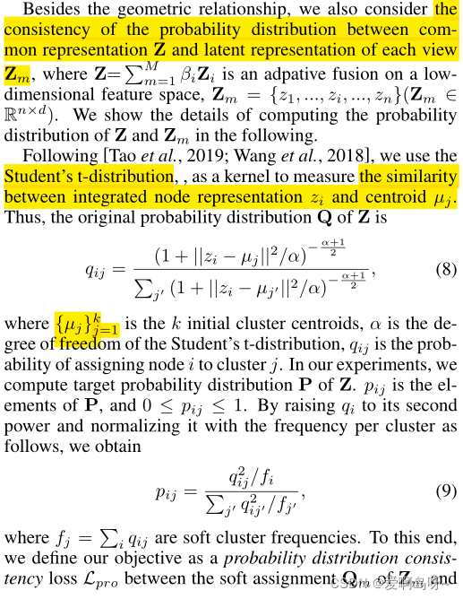
2.The consistency of the probability distribution

（就是让各个view下得到的概率分布矩阵都与总的概率分布矩阵去进行逼近，越逼近说明每个view下得到的概率分布矩阵都是比较好的，从而也说明了网络确实具有较好的鲁棒性。）
1.The auxiliary distribution $P$ of $Z$ with trade-off parameters $\rho$ as follows:
$$L_{pro}=\underset{\eta }{\min }\sum _{m=1}^M{\rho }_m||Q_m-P|{|}_F^2$$
2.计算细节：

（五）Task for Clustering

（用总的loss去不断优化网络，以此来达到我们之前分析的目的。）
1.The total loss function of the proposed MAGCN is eventully formulated as：
$$L=\underset{g,c,\mathbf{P}}{\min }{L}_{re}+{\lambda }_2{L}_{geo}+{\lambda }_3{L}_{pro}$$

2.Then we predict the cluster of each node from auxiliary distribution $P$. For node $i$, its cluster can be calculated by $p_i$ , in which the index with the highest probability value is the i’s cluster. Hence we could obtain the cluster label of node $i$ as:
$$y_i=\underset{k}{\mathrm{argmax}}{p}_{ik}$$