


💥💥💞💞欢迎来到本博客❤️❤️💥💥
🏆博主优势:🌞🌞🌞博客内容尽量做到思维缜密,逻辑清晰,为了方便读者。
⛳️座右铭:行百里者,半于九十。
📋📋📋本文目录如下:🎁🎁🎁
目录
💥1 概述
高斯Copula方法是一种用于建立多变量分布的方法,它可以将边缘分布和相关性结合起来,从而得到整体的联合分布。在这种方法中,边缘分布可以是任意的分布,而相关性则由Copula函数来描述。
首先,我们需要选择适当的Copula函数来描述变量之间的相关性。常用的Copula函数包括高斯Copula、t Copula、Clayton Copula等。在这里,我们选择高斯Copula作为例子来进行研究。
接下来,我们需要对相关参数进行迭代优化。一种常用的方法是最大似然估计,通过最大化似然函数来估计Copula函数的参数。通过迭代优化,我们可以得到最优的相关参数,从而得到最优的联合分布。
最后,我们可以利用得到的联合分布进行关联样本的生成。通过高斯Copula方法,我们可以生成符合指定边缘分布和相关性的样本,从而实现任意组合分布的关联样本生成。
基于高斯Copula方法对分布的任意组合进行关联样本,并对相关参数进行迭代优化是一种有效的研究方法,可以用于建立多变量分布的模型和生成关联样本。
一、高斯Copula方法的基本原理
1.1 数学定义与核心公式
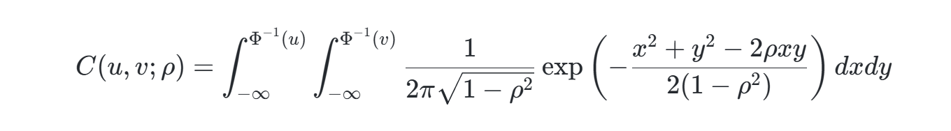
高斯Copula是基于多元正态分布构建的Copula函数,其核心思想是将边缘分布通过概率积分变换映射到标准正态空间,再利用协方差矩阵刻画变量间的依赖结构。对于d维随机变量,其联合分布函数定义为:

其中:
- ΦdΦd为d维标准正态分布的联合分布函数
- Φ−1Φ−1为标准正态分布的逆累积分布函数
- ΣΣ为相关系数矩阵(需满足正定性)
在双变量情形下,表达式可简化为:
1.2 与其他Copula的对比
| 特性 | 高斯Copula | t-Copula | Clayton Copula |
|---|---|---|---|
| 尾部依赖 | 无 | 对称尾部依赖 | 仅下尾依赖 |
| 参数范围 | ρ∈(−1,1) | ρ,ν>0 | θ∈(0,∞) |
| 适用场景 | 线性相关、对称分布 | 极端事件相关性 | 非对称风险传递 |
二、多分布组合建模方法
2.1 基于Sklar定理的建模流程
- 边缘分布选择:对每个变量XiXi独立拟合其边缘分布Fi(xi)Fi(xi)(如正态、指数、伽马等)。
- 概率积分变换:将原始数据转换为均匀分布Ui=Fi(Xi)Ui=Fi(Xi)。
- Copula参数估计:在均匀空间中估计相关系数矩阵ΣΣ,构建高斯Copula结构。
- 联合分布合成:通过F(x1,...,xd)=C(F1(x1),...,Fd(xd);Σ)F(x1,...,xd)=C(F1(x1),...,Fd(xd);Σ)生成联合分布。
2.2 特殊分布处理技巧
- 截断分布:对于有界分布(如截断正态),需调整概率积分变换的边界条件。
- 离散-连续混合:采用连续化方法(如jittering)处理离散变量,避免Copula密度不连续问题。
- 高维扩展:通过Vine Copula结构(如C-Vine、D-Vine)分层建模,降低维度灾难。
三、参数估计与迭代优化
3.1 最大似然估计(MLE)
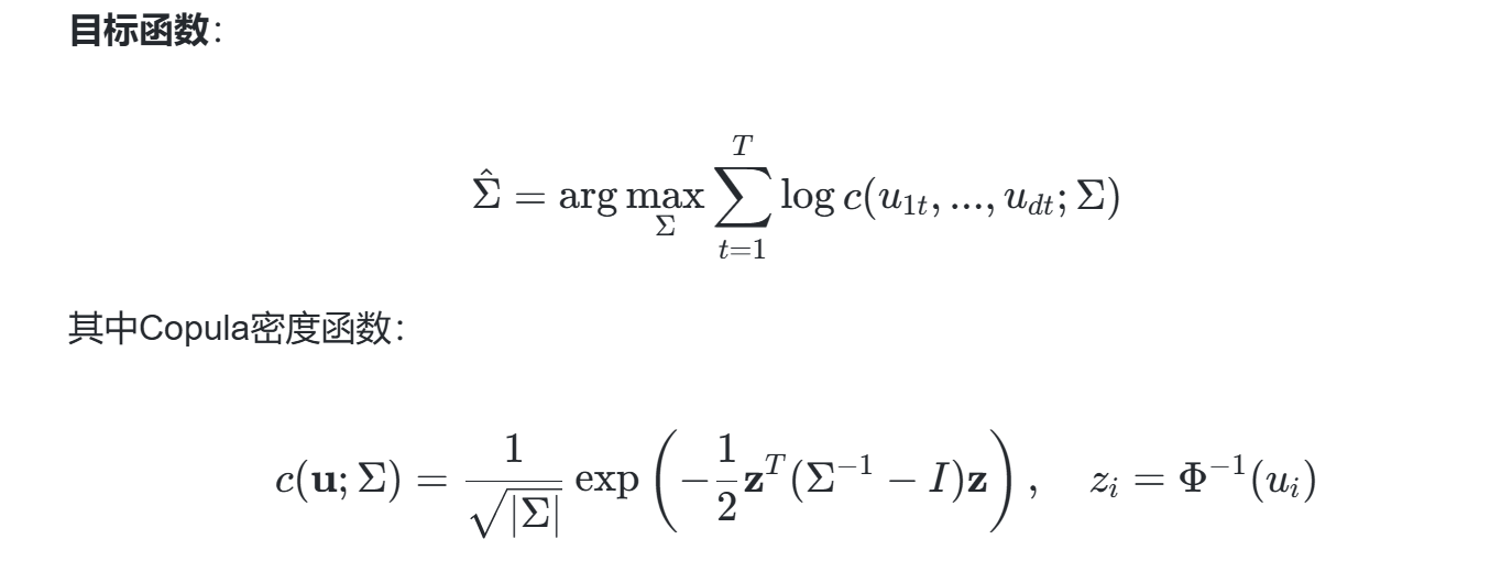
优化步骤:
- 初始化:使用Kendall's τ或Spearman's ρ计算初始相关系数。
- 梯度下降:采用拟牛顿法(如BFGS)迭代更新ΣΣ,确保正定性约束。
- 收敛判断:当参数变化量∥ΔΣ∥<ϵ或似然函数变化率低于阈值时终止。
3.2 两阶段估计法(IFM)

四、关联样本生成算法
4.1 蒙特卡洛模拟步骤

Matlab代码片段:
% 生成高斯Copula样本
Sigma = [1 0.5; 0.5 1]; % 相关系数矩阵
n = 1000; % 样本量
Z = mvnrnd([0,0], Sigma, n);
U = normcdf(Z);
X(:,1) = icdf('Normal', U(:,1), mu1, sigma1); % 边缘分布1
X(:,2) = icdf('Exponential', U(:,2), lambda); % 边缘分布2
4.2 动态参数优化案例
在金融风险管理中,通过滑动窗口法动态更新ΣΣ:
- 窗口划分:以30天为窗口,滚动更新历史数据。
- 参数估计:每个窗口内重新计算Σ^Σ^。
- 风险度量:计算动态VaR和ES,捕捉时变相关性。
五、应用场景与局限性
5.1 典型应用
- 金融工程:组合VaR计算、信用衍生品定价
- 能源系统:风电-光伏出力相关性建模
- 生物统计:病例对照研究中多表型关联分析
5.2 局限性及改进方向
| 局限性 | 改进方法 |
|---|---|
| 尾部独立性假设 | 混合t-Copula或Vine结构 |
| 高维参数估计困难 | 正则化(如Graphical Lasso) |
| 非线性依赖捕捉不足 | 核Copula或深度Copula |
结论:高斯Copula通过灵活的关联结构建模,为多变量分布分析提供了强大工具。结合参数迭代优化(如MLE、两阶段估计)和动态调整策略,可有效应对实际数据中的复杂依赖关系。未来研究可进一步探索其与机器学习模型的融合,提升在高维、非线性场景下的性能。
📚2 运行结果


部分代码:
function [funcVal, stdev, CI, MCfuncVals, MCsamples]= simulateMC(func,dists,N,varargin)
% simulateMC() is a tool for Monte Carlo simulation. It draws many, many
% samples from user-specified distributions and combines the samples through
% an arbitrary function.
% INPUTS:
% func Function handle of the function to combine samples through
% (func must be vectorizable so use .*, ./ and .^ instead of *, /, and ^)
% dists Vertical cell array of cell arrays containing params for each distribution
% N Number of samples to generate from each distribution
% 'CI',value (Optional) Value to use for pseudo CI threshold. Default is 0.68.
% 'hist',nBins (Optional) Plot histogram of the function outputs. nBins value is optional
% 'varHist',nBins (Optional) Plot histograms of each sample. nBins valueis optional.
% 'mean'|'median'|'max'|'min'
% (Optional) Specifies what value to return for 'funcVal'.
% Default is the center of the CI inteval.
%
% For each cell array inside 'dists' the syntax is:
% {'DistributionType',param_1,...,paramN[,'truncate',lowerBound,upperBound]}
% where the truncation arguments inside the square brackets are optional.
% OUTPUTS:
% funcVal Calculated function value. Defaults to center of CI. Can be mean, median, or max/min.
% stdev Standard deviation of the function outputs
% CI Vector containing the lowerbound and upperbound of the pseudo CI interval.
% (this is the shortest interval containing some percent of the function outputs)
% MCfuncVals Vector of the function outputs.
% MCsamples Array containing the samples for each distribution.
% %EXAMPLE 1
% %Combine samples from X and Y through the function 'f'.
% %'X' is a normal distribution with params [mean=5,sigma=1].
% %'Y' is a uniform distribution with params [lowerbound=6,upperbound=7].
% f=@(X,Y)5.*X+Y;
% dists = {{'Normal',5,1};
% {'Uniform',6,7}};
% n=100000;
% [funcVal,stdev,CI] = simulateMC(f,dists,n)
....
%% Parse varargin to handle optional arguments
%Init defaults
if (~exist('N', 'var'))
N=100000;
end
confInterval = 0.68;
meanFlag=0; medianFlag=0; maxFlag=0; minFlag=0;
histFlag=0; histBins=40;
varHistFlag = 0; varHistBins=40;
for vaIdx = 1:length(varargin)
currArg = varargin{vaIdx};
notLastArg = vaIdx~=length(varargin);
switch(currArg)
case {'mean','Mean'}
meanFlag=1;
case {'median','Median'}
medianFlag=1;
case {'max','Max'}
maxFlag=1;
case {'min','Min'}
minFlag=1;
case {'hist','Hist'}
histFlag=1;
if notLastArg && ~ischar(varargin{vaIdx+1})
histBins=varargin{vaIdx+1};
end
case {'varHist','VarHist','varhist','Varhist'}
varHistFlag=1;
if notLastArg && ~ischar(varargin{vaIdx+1})
varHistBins=varargin{vaIdx+1};
end
case {'CI','Ci','ci'}
if notLastArg && ~ischar(varargin{vaIdx+1})
confInterval=varargin{vaIdx+1};
else
disp('simulateMC(): Value is missing from ''CI'' name-value pair.')
end
otherwise
if ischar(currArg)
disp("simulateMC(): The string '"+currArg+"' in the function parameters was not recognized as a valid option.")
end
end
end
%% Generate & Store Samples From the Specified Distributions
distIdx=0;
sampIdx=0;
while(distIdx < size(dists,1))
distIdx=distIdx+1;
sampIdx=sampIdx+1;
distType = dists{distIdx}{1};
switch(distType)
case {'Bootstrap','bootstrap'}
%Bootstrap a sample of size N from user provided data.
%Syntax is: {'Bootstrap',datavec}
🎉3 参考文献
文章中一些内容引自网络,会注明出处或引用为参考文献,难免有未尽之处,如有不妥,请随时联系删除。
[1]杨柳.基于Copula函数的风—电—热相关性分析方法研究[D].东北电力大学,2020.
[2]王双成,高瑞,杜瑞杰.基于高斯Copula的约束贝叶斯网络分类器研究[J].计算机学报, 2016, 39(8):14.DOI:10.11897/SP.J.1016.2016.01612.


 1105
1105

 被折叠的 条评论
为什么被折叠?
被折叠的 条评论
为什么被折叠?
 到【灌水乐园】发言


