


本例使用的代价函数为
y
=
(
θ
−
2.5
)
2
−
1
y=(\theta - 2.5)^2-1
y=(θ−2.5)2−1,如果要使用其他代价函数,需要同时修改J(theta)和dJ(theta)函数
需要设置不同的学习率可以改变第71行函数传入参数
可以通过修改54行的epsilon来控制停止的时机
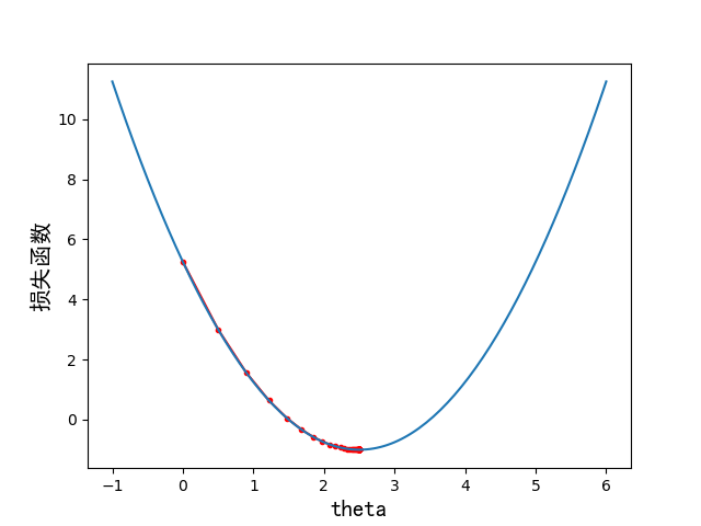
结果
学习率 η = 0.1 \eta = 0.1 η=0.1时:
共训练了46次
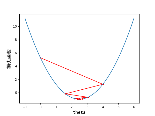
学习率 η = 0.8 \eta=0.8 η=0.8时:
共训练了22次
代码
# -*- coding:utf-8
"""
作者: Jia
日期: 2022年01月30日
描述: 梯度下降算法的实现
"""
import matplotlib.pyplot as plt
import numpy as np


def J(theta):
    """
    损失函数
    :param theta: 自变量值
    :return: 损失函数的值
    """
    return (theta - 2.5) ** 2 - 1


def dJ(theta):
    """
    损失函数的导数
    :param theta: 自变量值
    :return: 对应点处的导数值
    """
    return 2 * (theta - 2.5)


def plotJ(x, y, theta_history):
    """
    绘制代价函数的图形
    :param x: 横坐标
    :param y: 纵坐标
    :return: None
    """
    plt.plot(np.array(theta_history), J(np.array(theta_history)), color='r', marker='.')
    plt.plot(x, y)
    # 设置坐标轴名称
    plt.xlabel('theta', fontproperties='simHei', fontsize=15)
    plt.xlabel('损失函数', fontproperties='simHei', fontsize=15)
    plt.show()


def gradient_descent(eta):
    """
    梯度下降法求最优点
    :param eta: 学习率
    :return:
        theta: 最优点的取值
        theta_history: 学习过程中theta的取值
    """
    theta = 0.0
    theta_history = [theta]
    epsilon = 1e-8  # 当两次下降的差值小于该值时停止训练

    while True:
        gradient = dJ(theta)  # 求得该点处的导数值
        last_theta = theta
        theta = theta - eta * gradient  # 使用梯度下降计算新的theta
        theta_history.append(theta)  # 保留theta的取值,用于画图像
        if abs(J(theta) - J(last_theta)) < epsilon:
            break

    return theta, theta_history


if __name__ == '__main__':
    plot_x = np.linspace(-1, 6, 141)  # 取从-1到6的141个点
    plot_y = J(plot_x)  # 得到y坐标值

    theta, theta_history = gradient_descent(1.1)  # 在这里可以设置不同的学习率的取值
    plotJ(plot_x, plot_y, theta_history)  # 绘制代价函数图像
    print("共训练了", len(theta_history), "次")


 540
540


 被折叠的 条评论
为什么被折叠?
被折叠的 条评论
为什么被折叠?
 到【灌水乐园】发言


