


开源内容:https://github.com/TommyZihao/zihao_course/tree/main/CS224W
子豪兄B 站视频:https://space.bilibili.com/1900783/channel/collectiondetail?sid=915098
斯坦福官方课程主页:https://web.stanford.edu/class/cs224w
NetworkX主页:https://networkx.org
nx.Graph :https://networkx.org/documentation/stable/reference/classes/graph.html#networkx.Graph
给图、节点、连接添加属性:https://networkx.org/documentation/stable/tutorial.html#attributes
读写图:https://networkx.org/documentation/stable/reference/readwrite/index.html
文章目录
PageRank节点重要度
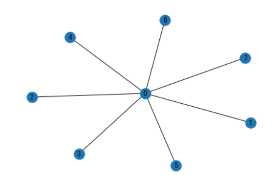
在NetworkX中,计算有向图节点的PageRank节点重要度。
# 图数据挖掘
import networkx as nx

# 数据可视化
import matplotlib.pyplot as plt
%matplotlib inline

plt.rcParams['font.sans-serif']=['SimHei']  # 用来正常显示中文标签
plt.rcParams['axes.unicode_minus']=False  # 用来正常显示负号
G = nx.star_graph(7)
nx.draw(G, with_labels = True)
pagerank = nx.pagerank(G, alpha=0.8)
pagerank
{0: 0.4583348922684132,
1: 0.07738072967594098,
2: 0.07738072967594098,
3: 0.07738072967594098,
4: 0.07738072967594098,
5: 0.07738072967594098,
6: 0.07738072967594098,
7: 0.07738072967594098}
节点连接数Node Degree度分析
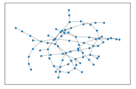
在NetworkX中,计算并统计图中每个节点的连接数Node Degree,绘制可视化和直方图。
# 图数据挖掘
import networkx as nx

import numpy as np

# 数据可视化
import matplotlib.pyplot as plt
%matplotlib inline

plt.rcParams['font.sans-serif']=['SimHei']  # 用来正常显示中文标签
plt.rcParams['axes.unicode_minus']=False  # 用来正常显示负号
# 创建 Erdős-Rényi 随机图,也称作 binomial graph
# n-节点数
# p-任意两个节点产生连接的概率

G = nx.gnp_random_graph(100, 0.02, seed=10374196)

# 初步可视化
pos = nx.spring_layout(G, seed=10)
nx.draw(G, pos)

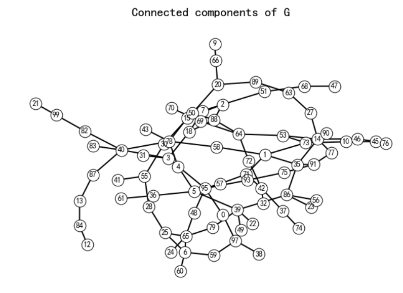
最大连通域子图
Gcc = G.subgraph(sorted(nx.connected_components(G), key=len, reverse=True)[0])
pos = nx.spring_layout(Gcc, seed=10396953)
# nx.draw(Gcc, pos)

nx.draw_networkx_nodes(Gcc, pos, node_size=20)
nx.draw_networkx_edges(Gcc, pos, alpha=0.4)
plt.figure(figsize=(12,8))
pos = nx.spring_layout(Gcc, seed=10396953)

# 设置其它可视化样式
options = {
    "font_size": 12,
    "node_size": 350,
    "node_color": "white",
    "edgecolors": "black",
    "linewidths": 1, # 节点线宽
    "width": 2, # edge线宽
}

nx.draw_networkx(Gcc, pos, **options)

plt.title('Connected components of G', fontsize=20)
plt.axis('off')
plt.show()
节点的连接数可视化
对节点按度的大小从大到小进行排列,绘制基本的点图
degree_sequence = sorted((d for n, d in G.degree()), reverse=True)
plt.figure(figsize=(12,8))
plt.plot(degree_sequence, "b-", marker="o")
plt.title('Degree Rank Plot', fontsize=20)
plt.ylabel('Degree', fontsize=25)
plt.xlabel('Rank', fontsize=25)
plt.tick_params(labelsize=20) # 设置坐标文字大小
plt.show()

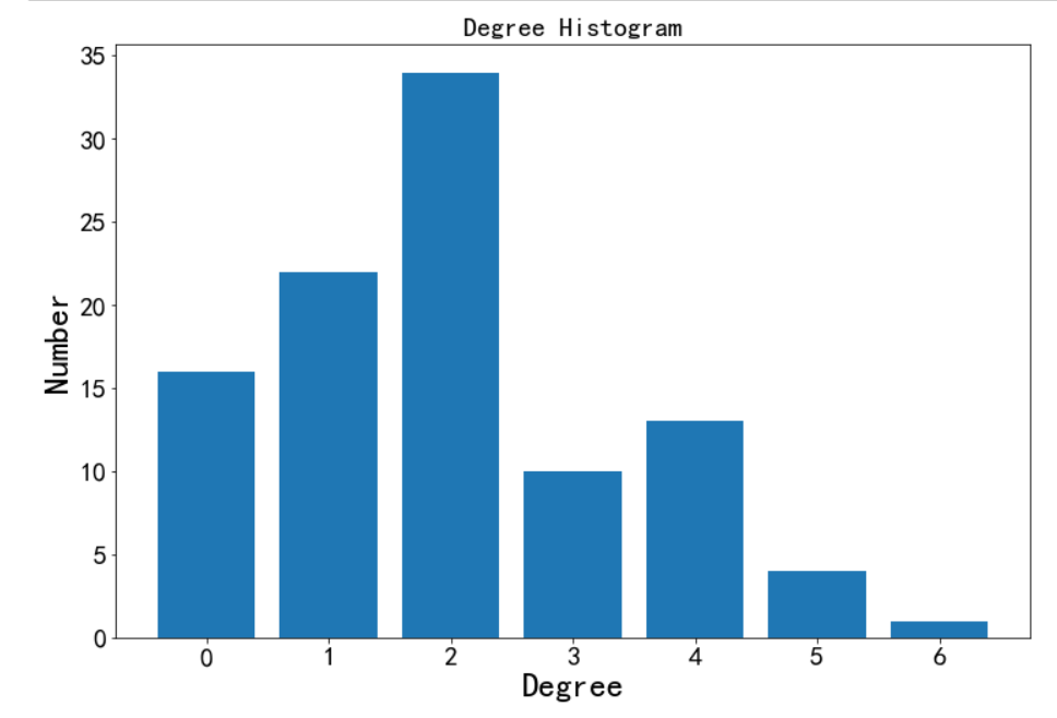
绘制直方图
X = np.unique(degree_sequence, return_counts=True)[0]
Y = np.unique(degree_sequence, return_counts=True)[1]

plt.figure(figsize=(12,8))
# plt.bar(*np.unique(degree_sequence, return_counts=True))
plt.bar(X, Y)

plt.title('Degree Histogram', fontsize=20)
plt.ylabel('Number', fontsize=25)
plt.xlabel('Degree', fontsize=25)
plt.tick_params(labelsize=20) # 设置坐标文字大小
plt.show()
plt.show()
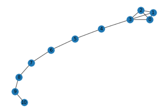
棒棒糖图特征分析
# 图数据挖掘
import networkx as nx

# 数据可视化
import matplotlib.pyplot as plt
%matplotlib inline

# plt.rcParams['font.sans-serif']=['SimHei']  # 用来正常显示中文标签
plt.rcParams['axes.unicode_minus']=False  # 用来正常显示负号
导入棒棒图
# 第一个参数指定头部节点数,第二个参数指定尾部节点数
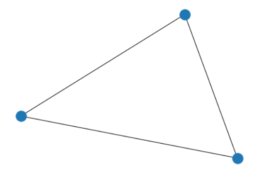
G = nx.lollipop_graph(4, 7)
pos = nx.spring_layout(G, seed=3068)
nx.draw(G, pos=pos, with_labels=True)
plt.show()
图数据分析
对图的基本特征进行分析,包括:半径、直径、偏心度、中心节点、外围节点、图的密度
在图的密度中:n为节点个数,m为连接个数
对于无向图:
d e n s i t y = 2 m n ( n − 1 ) density = \frac{2m}{n(n-1)} density=n(n−1)2m
对于有向图:
d e n s i t y = m n ( n − 1 ) density = \frac{m}{n(n-1)} density=n(n−1)m
无连接图的density为0,全连接图的density为1,Multigraph(多重连接图)和带self
loop图的density可能大于1。
# 半径
nx.radius(G)
# 直径
nx.diameter(G)
# 偏心度:每个节点到图中其它节点的最远距离
nx.eccentricity(G)
# 中心节点,偏心度与半径相等的节点
nx.center(G)
# 外围节点,偏心度与直径相等的节点
nx.periphery(G)
# 图的密度
nx.density(G)
每两个节点之间的最短距离
pathlengths = []
for v in G.nodes():
    spl = nx.single_source_shortest_path_length(G, v)
    for p in spl:
        print('{} --> {} 最短距离 {}'.format(v, p, spl[p]))
        pathlengths.append(spl[p])
# 平均最短距离
sum(pathlengths) / len(pathlengths)
不同距离的节点对个数
dist = {}
for p in pathlengths:
    if p in dist:
        dist[p] += 1
    else:
        dist[p] = 1
计算节点特征
计算无向图和有向图的节点特征。
import networkx as nx
import matplotlib.pyplot as plt
import matplotlib.colors as mcolors
%matplotlib inline
可视化辅助函数
def draw(G, pos, measures, measure_name):

    nodes = nx.draw_networkx_nodes(G, pos, node_size=250, cmap=plt.cm.plasma,
                                   node_color=list(measures.values()),
                                   nodelist=measures.keys())
    nodes.set_norm(mcolors.SymLogNorm(linthresh=0.01, linscale=1, base=10))
    # labels = nx.draw_networkx_labels(G, pos)
    edges = nx.draw_networkx_edges(G, pos)

    # plt.figure(figsize=(10,8))
    plt.title(measure_name)
    plt.colorbar(nodes)
    plt.axis('off')
    plt.show()
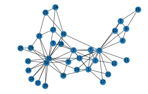
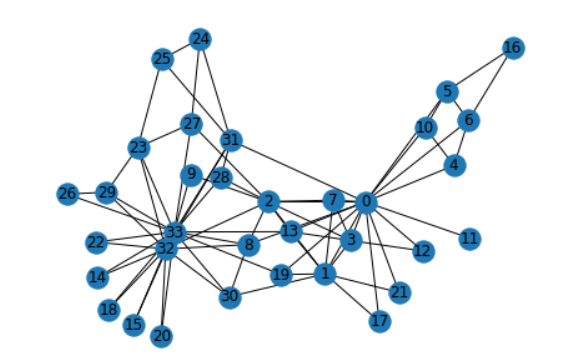
导入无向图
G = nx.karate_club_graph()
pos = nx.spring_layout(G, seed=675)
nx.draw(G, pos, with_labels=True)
导入有向图
DiG = nx.DiGraph()
DiG.add_edges_from([(2, 3), (3, 2), (4, 1), (4, 2), (5, 2), (5, 4),
                    (5, 6), (6, 2), (6, 5), (7, 2), (7, 5), (8, 2),
                    (8, 5), (9, 2), (9, 5), (10, 5), (11, 5)])
nx.draw(DiG, pos, with_labels=True)
Node Degree
list(nx.degree(G))

dict(G.degree())
# 字典按值排序
sorted(dict(G.degree()).items(),key=lambda x : x[1], reverse=True)
draw(G, pos, dict(G.degree()), 'Node Degree')
节点重要度特征 Centrality
https://networkx.org/documentation/stable/reference/algorithms/centrality.html
Degree Centrality
无向图
nx.degree_centrality(G)

draw(G, pos, nx.degree_centrality(G), 'Degree Centrality')
有向图
nx.in_degree_centrality(DiG)
nx.out_degree_centrality(DiG)

draw(DiG, pos, nx.in_degree_centrality(DiG), 'DiGraph Degree Centrality')
draw(DiG, pos, nx.out_degree_centrality(DiG), 'DiGraph Degree Centrality')
Eigenvector Centrality
无向图
nx.eigenvector_centrality(G)

draw(G, pos, nx.eigenvector_centrality(G), 'Eigenvector Centrality')
有向图
nx.eigenvector_centrality_numpy(DiG)

draw(DiG, pos, nx.eigenvector_centrality_numpy(DiG), 'DiGraph Eigenvector Centrality')
Betweenness Centrality(必经之地)
#nx.betweenness_centrality?
#nx.betweenness_centrality??
nx.betweenness_centrality(G)

draw(G, pos, nx.betweenness_centrality(G), 'Betweenness Centrality')
Closeness Centrality(去哪儿都近)
nx.closeness_centrality(G)

draw(G, pos, nx.closeness_centrality(G), 'Closeness Centrality')
PageRank
nx.pagerank(DiG, alpha=0.85)

draw(DiG, pos, nx.pagerank(DiG, alpha=0.85), 'DiGraph PageRank')
Katz Centrality
nx.katz_centrality(G, alpha=0.1, beta=1.0)

draw(G, pos, nx.katz_centrality(G, alpha=0.1, beta=1.0), 'Katz Centrality')
draw(DiG, pos, nx.katz_centrality(DiG, alpha=0.1, beta=1.0), 'DiGraph Katz Centrality')
HITS Hubs and Authorities
h, a = nx.hits(DiG)
draw(DiG, pos, h, 'DiGraph HITS Hubs')
draw(DiG, pos, a, 'DiGraph HITS Authorities')
社群属性 Clustering
https://networkx.org/documentation/stable/reference/algorithms/clustering.html
nx.draw(G, pos, with_labels=True)
三角形个数
nx.triangles(G)

draw(G, pos, nx.triangles(G), 'Triangles')
Clustering Coefficient
nx.clustering(G)
nx.clustering(G, 0)

draw(G, pos, nx.clustering(G), 'Clustering Coefficient')
Bridges
如果某个连接断掉,会使连通域个数增加,则该连接是bridge。
bridge连接不属于环的一部分。
pos = nx.spring_layout(G, seed=675)
nx.draw(G, pos, with_labels=True)
list(nx.bridges(G))
[(0, 11)]
Common Neighbors 、Jaccard Coefficient和Adamic-Adar index
基于两节点局部连接信息(Local neighborhood overlap)
pos = nx.spring_layout(G, seed=675)
nx.draw(G, pos, with_labels=True)
sorted(nx.common_neighbors(G, 0, 4))
preds = nx.jaccard_coefficient(G, [(0, 1), (2, 3)])
for u, v, p in preds:
    print(f"({u}, {v}) -> {p:.8f}")

for u, v, p in nx.adamic_adar_index(G, [(0, 1), (2, 3)]):
    print(f"({u}, {v}) -> {p:.8f}")
Katz Index
基于两节点在全图的连接信息(Global neighborhood overlap)
节点u到节点v,路径为k的路径个数。
import networkx as nx
import numpy as np
from numpy.linalg import inv
G = nx.karate_club_graph()

# 计算主特征向量
L = nx.normalized_laplacian_matrix(G)
e = np.linalg.eigvals(L.A)
print('最大特征值', max(e))

# 折减系数
beta = 1/max(e)

# 创建单位矩阵
I = np.identity(len(G.nodes))

# 计算 Katz Index
S = inv(I - nx.to_numpy_array(G)*beta) - I
array([[-0.630971 , 0.03760311, -0.50718655, …, 0.22028562,
0.08051109, 0.0187629 ],
[ 0.03760311, 0.0313979 , -1.09231501, …, 0.18920621,
-0.09098329, 0.08188737],
[-0.50718655, -1.09231501, 0.79993439, …, -0.4511988 ,
0.17631358, -0.23914987],
…,
[ 0.22028562, 0.18920621, -0.4511988 , …, -0.07349891,
0.47525815, -0.0457034 ],
[ 0.08051109, -0.09098329, 0.17631358, …, 0.47525815,
-0.28781332, -0.70104834],
[ 0.0187629 , 0.08188737, -0.23914987, …, -0.0457034 ,
-0.70104834, -0.50717615]])
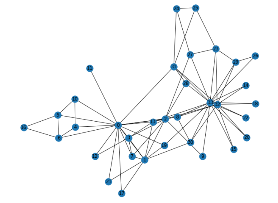
计算全图Graphlet个数
import networkx as nx
import matplotlib.pyplot as plt
%matplotlib inline

import itertools

G = nx.karate_club_graph()
plt.figure(figsize=(10,8))
pos = nx.spring_layout(G, seed=123)
nx.draw(G, pos, with_labels=True)
指定Graphlet
target = nx.complete_graph(3)
nx.draw(target)
匹配Graphlet,统计个数
num = 0
for sub_nodes in itertools.combinations(G.nodes(), len(target.nodes())):  # 遍历全图中,符合graphlet节点个数的所有节点组合
    subg = G.subgraph(sub_nodes)                                          # 从全图中抽取出子图
    if nx.is_connected(subg) and nx.is_isomorphic(subg, target):          # 如果子图是完整连通域,并且符合graphlet特征,输出原图节点编号
        num += 1
        print(subg.edges())
num
拉普拉斯矩阵特征值分解
# 图数据挖掘
import networkx as nx

import numpy as np

# 数据可视化
import matplotlib.pyplot as plt
%matplotlib inline

plt.rcParams['font.sans-serif']=['SimHei']  # 用来正常显示中文标签
plt.rcParams['axes.unicode_minus']=False  # 用来正常显示负号

import numpy.linalg # 线性代数
创建图
n = 1000  # 节点个数
m = 5000  # 连接个数
G = nx.gnm_random_graph(n, m, seed=5040)
邻接矩阵(Adjacency Matrix)
A = nx.adjacency_matrix(G)
A.todense()
matrix([[0, 0, 0, …, 0, 0, 0],
[0, 0, 0, …, 0, 0, 0],
[0, 0, 0, …, 0, 0, 0],
…,
[0, 0, 0, …, 0, 0, 0],
[0, 0, 0, …, 0, 0, 0],
[0, 0, 0, …, 0, 0, 0]], dtype=int32)
拉普拉斯矩阵(Laplacian Matrix)
L = D − A L = D - A L=D−A
L 为拉普拉斯矩阵(Laplacian Matrix)
D 为节点degree对角矩阵
A 为邻接矩阵(Adjacency Matrix)
L = nx.laplacian_matrix(G)
# 节点degree对角矩阵
D = L + A
D.todense()
matrix([[12, 0, 0, …, 0, 0, 0],
[ 0, 6, 0, …, 0, 0, 0],
[ 0, 0, 8, …, 0, 0, 0],
…,
[ 0, 0, 0, …, 8, 0, 0],
[ 0, 0, 0, …, 0, 6, 0],
[ 0, 0, 0, …, 0, 0, 7]], dtype=int64)
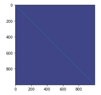
归一化拉普拉斯矩阵(Normalized Laplacian Matrix)
L n = D − 1 2 L D − 1 2 L_n = D^{-\frac{1}{2}}LD^{-\frac{1}{2}} Ln=D−21LD−21
L_n = nx.normalized_laplacian_matrix(G)
L_n.todense()

plt.imshow(L_n.todense())
plt.show()
特征值分解
e = np.linalg.eigvals(L_n.A)
# 最大特征值
max(e)
# 最小特征值
min(e)
特征值分布直方图
plt.figure(figsize=(12,8))

plt.hist(e, bins=100)
plt.xlim(0, 2)  # eigenvalues between 0 and 2

plt.title('Eigenvalue Histogram', fontsize=20)
plt.ylabel('Frequency', fontsize=25)
plt.xlabel('Eigenvalue', fontsize=25)
plt.tick_params(labelsize=20) # 设置坐标文字大小
plt.show()

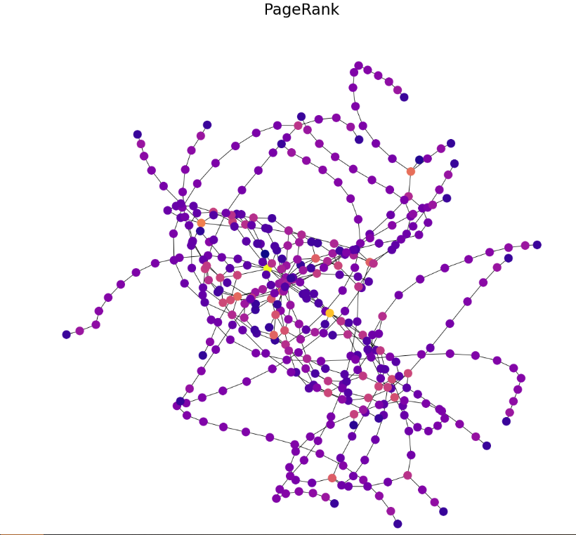
北京上海地铁站图数据挖掘
上海、北京地铁站点图数据挖掘,计算地铁站点的最短路径、节点重要度、集群系数、连通性。
import networkx as nx
import pandas as pd
import matplotlib.pyplot as plt
import matplotlib.colors as mcolors
%matplotlib inline
可视化辅助函数
def draw(G, pos, measures, measure_name):

    plt.figure(figsize=(20, 20))
    nodes = nx.draw_networkx_nodes(G, pos, node_size=250, cmap=plt.cm.plasma,
                                   node_color=list(measures.values()),
                                   nodelist=measures.keys())
    nodes.set_norm(mcolors.SymLogNorm(linthresh=0.01, linscale=1, base=10))
    # labels = nx.draw_networkx_labels(G, pos)
    edges = nx.draw_networkx_edges(G, pos)

    plt.title(measure_name, fontsize=30)
    # plt.colorbar(nodes)
    plt.axis('off')
    plt.show()
字典按值排序辅助函数
def dict_sort_by_value(dict_input):
    '''
    输入字典,输出按值排序的字典
    '''
    return sorted(dict_input.items(),key=lambda x : x[1], reverse=True)
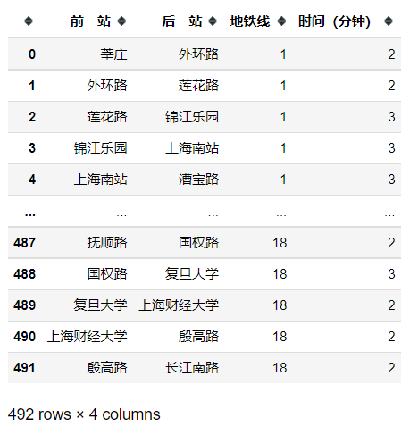
导入地铁站连接表
数据来源:
上海地铁线路图:http://www.shmetro.com
上海地铁时刻表:http://service.shmetro.com/hcskb/index.htm
北京地铁线路图:https://map.bjsubway.com
北京地铁时刻表:https://www.bjsubway.com/station/smcsj
# 上海地铁站点连接表
df = pd.read_csv('shanghai_subway.csv')

# 北京地铁站点连接表
# df = pd.read_csv('beijing_subway.csv')
df
创建图
# 创建无向图
G = nx.Graph()

# 从连接表创建图
for idx, row in df.iterrows(): # 遍历表格的每一行
    G.add_edges_from([(row['前一站'], row['后一站'])], line=row['地铁线'], time=row['时间(分钟)'])
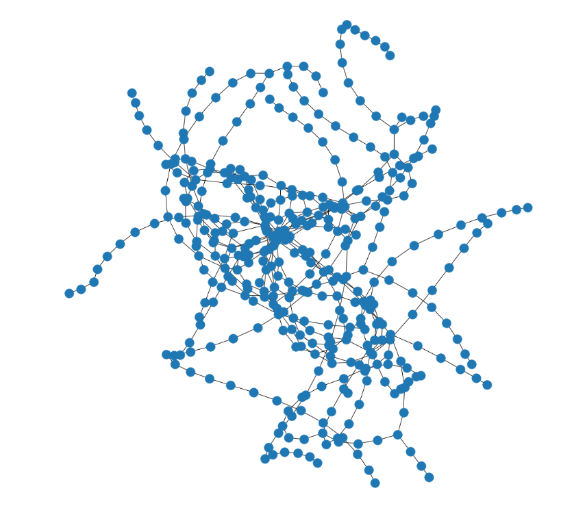
可视化
# 节点排版布局-默认弹簧布局
pos = nx.spring_layout(G, seed=123)

# 节点排版布局-每个节点单独设置坐标
# pos = {1: [0.1, 0.9], 2: [0.4, 0.8], 3: [0.8, 0.9], 4: [0.15, 0.55],
#         5: [0.5,  0.5], 6: [0.8,  0.5], 7: [0.22, 0.3], 8: [0.30, 0.27],
#         9: [0.38, 0.24], 10: [0.7,  0.3], 11: [0.75, 0.35]}
plt.figure(figsize=(15,15))
nx.draw(G, pos=pos)
Shortest Path 最短路径
NetworkX-最短路径算法:https://networkx.org/documentation/stable/reference/algorithms/shortest_paths.html
# 任意两节点之间是否存在路径
nx.has_path(G, source='昌吉东路', target='同济大学')

# 任意两节点之间的最短路径
nx.shortest_path(G, source='昌吉东路', target='同济大学', weight='time')

# 任意两节点之间的最短路径长度
nx.shortest_path_length(G, source='昌吉东路', target='同济大学', weight='time')

# 全图平均最短路径
nx.average_shortest_path_length(G, weight='time')

# 某一站去其他站的最短路径
nx.single_source_shortest_path(G, source='同济大学')

#某一站去其他站的最短路径长度
nx.single_source_shortest_path_length(G, source='同济大学')
地图导航系统
# 指定起始站和终点站
A_station = '昌吉东路'
B_station = '同济大学'

# 获取最短路径
shortest_path_list = nx.shortest_path(G, source=A_station, target=B_station, weight='time')

for i in range(len(shortest_path_list)-1):
    previous_station = shortest_path_list[i]
    next_station = shortest_path_list[i+1]
    line_id = G.edges[(previous_station, next_station)]['line'] # 地铁线编号
    time = G.edges[(previous_station, next_station)]['time']    # 时间
    print('{}--->{} {}号线 {}分钟'.format(previous_station, next_station, line_id, time)) # 输出结果

# 最短路径长度
print('共计 {} 分钟'.format(nx.shortest_path_length(G, source=A_station, target=B_station, weight='time')))
昌吉东路—>上海赛车场 11号线 4分钟
上海赛车场—>嘉定新城 11号线 4分钟
嘉定新城—>马陆 11号线 3分钟
马陆—>陈翔公路 11号线 4分钟
陈翔公路—>南翔 11号线 3分钟
南翔—>桃浦新村 11号线 3分钟
桃浦新村—>武威路 11号线 3分钟
武威路—>祁连山路 11号线 2分钟
祁连山路—>李子园 11号线 3分钟
李子园—>上海西站 11号线 2分钟
上海西站—>真如 11号线 3分钟
真如—>枫桥路 11号线 2分钟
枫桥路—>曹杨路 11号线 2分钟
曹杨路—>镇坪路 4号线 3分钟
镇坪路—>中潭路 4号线 2分钟
中潭路—>上海火车站 4号线 3分钟
上海火车站—>宝山路 4号线 4分钟
宝山路—>海伦路 4号线 3分钟
海伦路—>邮电新村 10号线 2分钟
邮电新村—>四平路 10号线 2分钟
四平路—>同济大学 10号线 2分钟
共计 59 分钟
PageRank
draw(G, pos, nx.pagerank(G, alpha=0.85), 'PageRank')
同样我们也可以计算节点的其它特征
总结
本篇文章主要介绍了NetworkX工具包实战在特征工程上的使用,利用NetworkX工具包对节点的度、节点重要度特征 、社群属性和等算法和拉普拉斯矩阵特征值分解等进行了计算,最后对北京上海地铁站图数据进行了挖掘。


 506
506


 被折叠的 条评论
为什么被折叠?
被折叠的 条评论
为什么被折叠?
 到【灌水乐园】发言


