基于kalman的单目标追踪，以及demo测试（Python and C++）

nice-wyh

已于 2024-03-29 18:40:38 修改

阅读量1.1k

点赞数 29

文章标签： python 开发语言算法 c++

于 2024-03-29 15:32:23 首次发布

本文链接：https://blog.csdn.net/qq_46454669/article/details/137143360

版权

一.卡尔曼滤波简单介绍

我们可以在任何含有不确定信息的动态系统中的使用卡尔曼滤波，对系统的下一步动作做出有根据的猜测。猜测的依据是预测值和观测值，首先我们认为预测值和观测值都符合高斯分布且包含误差，然后我们预设预测值的误差Q和观测值的误差R，然后计算得到卡尔曼增益，最后利用卡尔曼增益来综合预测值和观测值的结果，得到我们要的最优估计。通俗的说卡尔曼滤波就是将算出来的预测值和观测值综合考虑的过程。

二.主要公式

卡尔曼滤波器的推导过程比较复杂，这里不展开，这篇文章讲推导过程很好，下面5个公式是卡尔曼滤波器的核心，掌握了这5个公式，就基本掌握了卡尔曼滤波器的大致原理，下面只给出卡尔曼增益的推导过程。

首先给定一个系统，可以写出他的状态方程和观测方程，即为

状态方程： $x_{k} =Ax_{k-1}+B u_{k-1}+w_{k-1}$
观测方程： $z_{k} =Hx_{k}+v_{k}$

几个名词解释：

预测值：根据上一次最优估计而计算出来的值。

观测值：很好理解，就是观测到的值，比如观测到的物体的位置、速度。

最优估计：又叫后验状态估计值，滤波器的最终输出，也作为下一次迭代的输入。

卡尔曼滤波器最核心的5个公式：

预测

1.状态预测公式，作用是根据上一轮的最优估计，计算本轮的预测值

$\hat{x}_{k}^{-} =A\hat{x} _{k-1} +Bu _{k-1}$

其中A称为状态转移矩阵，表示我们如何从上一状态推测出当前状态；B表示控制矩阵，表示控制量u对当前状态的影响；u表示控制量，比如加速度；x头上之所以加一个^表示它是一个估计值，而不是真实值，而-上标表示这并非最佳估计。

2.噪声协方差公式，表示不确定性在各个时刻之间的传递关系，作用是计算本轮预测值的系统噪声协方差矩阵。

$P_{k}^{-} =AP _{k-1}A^{T} +Q$

A表示状态转移矩阵，P为系统噪声协方差矩阵（即每次的预测值和上一次最优估计误差的协方差矩阵,初始化时设置为E），Q为表示误差的矩阵

更新

3.计算K卡尔曼系数，又叫卡尔曼增益。

$K_{k} =P_{k}^{-}H^{T} (HP_{k}^{-}H^{T}+R)^{-1}$

H表示观测矩阵，R表示观测噪声的协方差矩阵

卡尔曼系数的作用主要有两个方面：

第一是权衡预测状态协方差矩阵P和观察量协方差矩阵R的大小，来决定我们是相信预测模型多一点还是观察模型多一点。如果相信预测模型多一点，这个残差的权重就会小一点，如果相信观察模型多一点，权重就会大一点。

第二就是把残差的表现形式从观察域转换到状态域，在我们这个例子中，观察值z表示的是小车的位置，只是一个一维向量，而状态向量是一个二维向量，它们所使用的单位和描述的特征都是不同的。而卡尔曼系数就是要实现这样将一维的观测向量转换为二维的状态向量的残差，在本例中我们只观测了小车的位置，而在K中已经包含了协方差矩阵P的信息，所以就利用了位置和速度这两个维度的相关性，从位置的信息中推测出了速度的信息，从而让我们可以对状态量x的两个维度同时进行修正。

4.最优估计公式，作用是利用观测值和预测值的残差对当前预测值进行调整，用的就是加权求和的方式。

$\hat{x} _{k}=\hat{x} _{k}^{-}+K_{k}(Z_{k}-H\hat{x} _{k}^{-})$

z是观测值，K是卡尔曼系数。

5.更新过程噪声协方差矩阵，下一次迭代中2式使用。

$P _{k}=(I-K_{k}H)\hat{x} _{k}^{-}+P_{k}^{-}$

三.基于python的单个行人demo

在正常的跟踪任务里，我们使用iou匹配 里面用到了上一帧的检测框来对下一帧进行iou计算来匹配(取最大值），但是呢，iou匹配一旦找不到最大值就会失去匹配目标，也就是会出现因为遮挡产生的lost(漏检)，所以引入卡尔曼滤波之后可以让上一帧的检测框具有运动属性(例如，框的dx,dy),从而使得最终的框不再和之前一样来自于上一帧，而是根据运动属性预测下一帧，保持和当前检测框处于同一时间，从而解决iou匹配的问题。

代码

基于此，有了如下的代码

import os
import cv2
import numpy as np
from utils import plot_one_box, cal_iou, xyxy_to_xywh, xywh_to_xyxy, updata_trace_list, draw_trace

# 单目标跟踪
# 检测器获得检测框，全程只赋予1个ID，有两个相同的东西进来时，不会丢失唯一跟踪目标
# 检测器的检测框为测量值
# 目标的状态X = [x,y,h,w,delta_x,delta_y],中心坐标，宽高，中心坐标速度
# 观测值
# 如何寻找目标的观测值
# 观测到的是N个框
# 怎么找到目标的观测值
# t时刻的框与t-1后验估计时刻IOU最大的框的那个作为观测值（存在误差，交叉情况下观测值会有误差）
# 所以需要使用先验估计值进行融合
#

# 状态初始化
initial_target_box = [729, 238, 764, 339]  # 目标初始bouding box
# initial_target_box = [193 ,342 ,250 ,474]

initial_box_state = xyxy_to_xywh(initial_target_box)
initial_state = np.array([[initial_box_state[0], initial_box_state[1], initial_box_state[2], initial_box_state[3],
                           0, 0]]).T  # [中心x,中心y,宽w,高h,dx,dy]
IOU_Threshold = 0.3 # 匹配时的阈值

# 状态转移矩阵，上一时刻的状态转移到当前时刻
A = np.array([[1, 0, 0, 0, 1, 0],
              [0, 1, 0, 0, 0, 1],
              [0, 0, 1, 0, 0, 0],
              [0, 0, 0, 1, 0, 0],
              [0, 0, 0, 0, 1, 0],
              [0, 0, 0, 0, 0, 1]])


# 状态观测矩阵
H = np.eye(6)

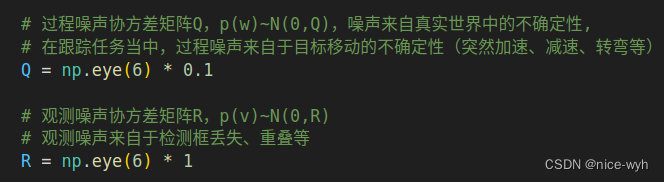
# 过程噪声协方差矩阵Q，p(w)~N(0,Q)，噪声来自真实世界中的不确定性,
# 在跟踪任务当中，过程噪声来自于目标移动的不确定性（突然加速、减速、转弯等）
Q = np.eye(6) * 0.1

# 观测噪声协方差矩阵R，p(v)~N(0,R)
# 观测噪声来自于检测框丢失、重叠等
R = np.eye(6) * 1

# 控制输入矩阵B
B = None
# 状态估计协方差矩阵P初始化
P = np.eye(6)

if __name__ == "__main__":

    video_path = "./data/testvideo1.mp4"
    label_path = "./data/labels"
    file_name = "testvideo1"
    cap = cv2.VideoCapture(video_path)
    # cv2.namedWindow("track", cv2.WINDOW_NORMAL)
    SAVE_VIDEO = False
    if SAVE_VIDEO:
        fourcc = cv2.VideoWriter_fourcc(*'XVID')
        out = cv2.VideoWriter('kalman_output.avi', fourcc, 20,(768,576))

    # ---------状态初始化----------------------------------------
    frame_counter = 1
    X_posterior = np.array(initial_state)
    P_posterior = np.array(P)
    Z = np.array(initial_state)
    trace_list = []  # 用于保存目标box的轨迹

    while (True):
        # Capture frame-by-frame
        ret, frame = cap.read()

        last_box_posterior = xywh_to_xyxy(X_posterior[0:4])
        plot_one_box(last_box_posterior, frame, color=(255, 255, 255), target=False)
        if not ret:
            break
        # print(frame_counter)
        label_file_path = os.path.join(label_path, file_name + "_" + str(frame_counter) + ".txt")
        with open(label_file_path, "r") as f:
            content = f.readlines()
            max_iou = IOU_Threshold
            max_iou_matched = False
            # ---------使用最大IOU来寻找观测值------------
            for j, data_ in enumerate(content):
                data = data_.replace('\n', "").split(" ")
                xyxy = np.array(data[1:5], dtype="float")
                plot_one_box(xyxy, frame)
                iou = cal_iou(xyxy, xywh_to_xyxy(X_posterior[0:4]))
                if iou > max_iou:
                    target_box = xyxy
                    max_iou = iou
                    max_iou_matched = True
            if max_iou_matched == True:
                # 如果找到了最大IOU BOX,则认为该框为观测值
                plot_one_box(target_box, frame, target=True)
                xywh = xyxy_to_xywh(target_box)
                box_center = (int((target_box[0] + target_box[2]) // 2), int((target_box[1] + target_box[3]) // 2))
                trace_list = updata_trace_list(box_center, trace_list, 100)
                cv2.putText(frame, "Tracking", (int(target_box[0]), int(target_box[1] - 5)), cv2.FONT_HERSHEY_SIMPLEX,
                            0.7,
                            (255, 0, 0), 2)
                # 计算dx,dy
                dx = xywh[0] - X_posterior[0]
                dy = xywh[1] - X_posterior[1]

                Z[0:4] = np.array([xywh]).T
                Z[4::] = np.array([dx, dy])

        if max_iou_matched:
            # -----进行先验估计-----------------
            X_prior = np.dot(A, X_posterior)
            box_prior = xywh_to_xyxy(X_prior[0:4])
            # plot_one_box(box_prior, frame, color=(0, 0, 0), target=False)
            # -----计算状态估计协方差矩阵P--------
            P_prior_1 = np.dot(A, P_posterior)
            P_prior = np.dot(P_prior_1, A.T) + Q
            # ------计算卡尔曼增益---------------------
            k1 = np.dot(P_prior, H.T)
            k2 = np.dot(np.dot(H, P_prior), H.T) + R
            K = np.dot(k1, np.linalg.inv(k2))
            # --------------后验估计------------
            X_posterior_1 = Z - np.dot(H, X_prior)
            X_posterior = X_prior + np.dot(K, X_posterior_1)
            box_posterior = xywh_to_xyxy(X_posterior[0:4])
            # plot_one_box(box_posterior, frame, color=(255, 255, 255), target=False)
            # ---------更新状态估计协方差矩阵P-----
            P_posterior_1 = np.eye(6) - np.dot(K, H)
            P_posterior = np.dot(P_posterior_1, P_prior)
        else:
            # 如果IOU匹配失败，此时失去观测值，那么直接使用上一次的最优估计作为先验估计
            # 此时直接迭代，不使用卡尔曼滤波
            X_posterior = np.dot(A, X_posterior)
            # X_posterior = np.dot(A_, X_posterior)
            box_posterior = xywh_to_xyxy(X_posterior[0:4])
            # plot_one_box(box_posterior, frame, color=(255, 255, 255), target=False)
            box_center = (
            (int(box_posterior[0] + box_posterior[2]) // 2), int((box_posterior[1] + box_posterior[3]) // 2))
            trace_list = updata_trace_list(box_center, trace_list, 20)
            cv2.putText(frame, "Lost", (box_center[0], box_center[1] - 5), cv2.FONT_HERSHEY_SIMPLEX, 0.7,
                        (255, 0, 0), 2)

        draw_trace(frame, trace_list)


        cv2.putText(frame, "ALL BOXES(Green)", (25, 50), cv2.FONT_HERSHEY_SIMPLEX, 0.7, (0, 200, 0), 2)
        cv2.putText(frame, "TRACKED BOX(Red)", (25, 75), cv2.FONT_HERSHEY_SIMPLEX, 0.7, (0, 0, 255), 2)
        cv2.putText(frame, "Last frame best estimation(White)", (25, 100), cv2.FONT_HERSHEY_SIMPLEX, 0.7, (255, 255, 255), 2)

        cv2.imshow('track', frame)
        if SAVE_VIDEO:
            out.write(frame)
        frame_counter = frame_counter + 1
        if cv2.waitKey(10) & 0xFF == ord('q'):
            break

    # When everything done, release the capture
    cap.release()
    cv2.destroyAllWindows()

    # 关注我
    # 你关注我了吗
    # 关注一下

其中的utils.py为

import cv2

def xyxy_to_xywh(xyxy):
    center_x = (xyxy[0] + xyxy[2]) / 2
    center_y = (xyxy[1] + xyxy[3]) / 2
    w = xyxy[2] - xyxy[0]
    h = xyxy[3] - xyxy[1]
    return (center_x, center_y, w, h)

def plot_one_box(xyxy, img, color=(0, 200, 0), target=False):
    xy1 = (int(xyxy[0]), int(xyxy[1]))
    xy2 = (int(xyxy[2]), int(xyxy[3]))
    if target:
        color = (0, 0, 255)
    cv2.rectangle(img, xy1, xy2, color, 1, cv2.LINE_AA)  # filled


def updata_trace_list(box_center, trace_list, max_list_len=50):
    if len(trace_list) <= max_list_len:
        trace_list.append(box_center)
    else:
        trace_list.pop(0)
        trace_list.append(box_center)
    return trace_list


def draw_trace(img, trace_list):
    """
    更新trace_list,绘制trace
    :param trace_list:
    :param max_list_len:
    :return:
    """
    for i, item in enumerate(trace_list):

        if i < 1:
            continue
        cv2.line(img,
                 (trace_list[i][0], trace_list[i][1]), (trace_list[i - 1][0], trace_list[i - 1][1]),
                 (255, 255, 0), 3)


def cal_iou(box1, box2):
    """

    :param box1: xyxy 左上右下
    :param box2: xyxy
    :return:
    """
    x1min, y1min, x1max, y1max = box1[0], box1[1], box1[2], box1[3]
    x2min, y2min, x2max, y2max = box2[0], box2[1], box2[2], box2[3]
    # 计算两个框的面积
    s1 = (y1max - y1min + 1.) * (x1max - x1min + 1.)
    s2 = (y2max - y2min + 1.) * (x2max - x2min + 1.)

    # 计算相交部分的坐标
    xmin = max(x1min, x2min)
    ymin = max(y1min, y2min)
    xmax = min(x1max, x2max)
    ymax = min(y1max, y2max)

    inter_h = max(ymax - ymin + 1, 0)
    inter_w = max(xmax - xmin + 1, 0)

    intersection = inter_h * inter_w
    union = s1 + s2 - intersection

    # 计算iou
    iou = intersection / union
    return iou


def cal_distance(box1, box2):
    """
    计算两个box中心点的距离
    :param box1: xyxy 左上右下
    :param box2: xyxy
    :return:
    """
    center1 = ((box1[0] + box1[2]) // 2, (box1[1] + box1[3]) // 2)
    center2 = ((box2[0] + box2[2]) // 2, (box2[1] + box2[3]) // 2)
    dis = ((center1[0] - center2[0]) ** 2 + (center1[1] - center2[1]) ** 2) ** 0.5

    return dis


def xywh_to_xyxy(xywh):
    x1 = xywh[0] - xywh[2]//2
    y1 = xywh[1] - xywh[3]//2
    x2 = xywh[0] + xywh[2] // 2
    y2 = xywh[1] + xywh[3] // 2

    return [x1, y1, x2, y2]


if __name__ == "__main__":
    box1 = [100, 100, 200, 200]
    box2 = [100, 100, 200, 300]
    iou = cal_iou(box1, box2)
    print(iou)
    box1.pop(0)
    box1.append(555)
    print(box1)

完成代码链接：链接: https://pan.baidu.com/s/11hBNOpZVNojYgD5awcsTgg?pwd=vxtv 提取码: vxtv 复制这段内容后打开百度网盘手机App，操作更方便哦

简单解读一下：

在这个代码里，我们设置了系统状态为X=[x, y, w, h, dx, dy],

状态转移矩阵A= $\begin{pmatrix} 1 & 0&0 & 0& 1& 0\\ 0 & 1& 0 & 0& 0& 1\\ 0& 0& 1& 0& 0& 0\\ 0& 0& 0& 1& 0& 0\\ 0& 0& 0& 0& 1& 0\\ 0& 0& 0& 0 & 0&1 \end{pmatrix}$ ，控制输入矩阵B=0（零矩阵）

状态观测矩阵H=E= $\begin{pmatrix} 1 & 0&0 & 0& 0& 0\\ 0 & 1& 0 & 0& 0& 0\\ 0& 0& 1& 0& 0& 0\\ 0& 0& 0& 1& 0& 0\\ 0& 0& 0& 0& 1& 0\\ 0& 0& 0& 0 & 0&1 \end{pmatrix}$

其中过程噪声p(w)~N(0, Q),来自于目标移动的不确定性，Q叫做误差的矩阵

观测噪声p(v)~N(0, R)，来自于检测框的丢失，重叠，不确定，R叫做观测噪声的协方差矩阵

同时在代码里，通过调节R和Q（即代码里的*0.1和*1）来选择更相信预测值还是更相信观测值，很明显，由于在单目标跟踪任务中，检测框的重叠和丢失是致命的，而目标的移动多为线性的，所以观测噪声p(v)~N(0, R) >> 过程噪声p(w)~N(0, Q)

所以，这里取Q为*0.1和R为*1

放上图片的解释

效果演示

只使用最大IOU的效果

maxiou output

使用kalman的效果

kalman_output

扩展

以上代码使用的系统状态为X=[x, y, w, h, dx, dy],我们可以改为8states的方式来改善跟踪效果（一般的六维数据就已经够了，这里只做演示），

即系统状态为X=[x, y, w, h, dx,dy,dw,dh]，相应的

状态转移矩阵A= $\begin{pmatrix} 1 &0 &0 &0 &1 &0 &0 &0 \\ 0& 1 & 0 & 0 &0 &1 &0 &0 \\ 0& 0 &1 & 0 & 0 &0 &1 &0 \\ 0& 0 & 0 & 1 &0 &0 &0 &1 \\ 0 & 0 & 0 & 0 &1 &0 &0 &0 \\ 0 & 0 &0 & 0&0 &1 & 0&0 \\ 0& 0 & 0 & 0 & 0 & 0 & 1 & 0\\ 0&0 & 0&0 & 0& 0&0 &1 \end{pmatrix}$ 控制输入矩阵B=0（零矩阵）

状态观测矩阵H=E= $\begin{pmatrix} 1 &0 &0 &0 &0 &0 &0 &0 \\ 0& 1 & 0 & 0 &0 &0 &0 &0 \\ 0& 0 &1 & 0 & 0 &0 &0 &0 \\ 0& 0 & 0 & 1 &0 &0 &0 &0 \\ 0 & 0 & 0 & 0 &1 &0 &0 &0 \\ 0 & 0 &0 & 0&0 &1 & 0&0 \\ 0& 0 & 0 & 0 & 0 & 0 & 1 & 0\\ 0&0 & 0&0 & 0& 0&0 &1 \end{pmatrix}$

代码为

import os
import cv2
import numpy as np
from utils import plot_one_box, cal_iou, xyxy_to_xywh, xywh_to_xyxy, updata_trace_list, draw_trace

# 单目标跟踪
# 检测器获得检测框，全程只赋予1个ID，有两个相同的东西进来时，不会丢失唯一跟踪目标
# 检测器的检测框为测量值
# 目标的状态X = [x,y,h,w,delta_x,delta_y],中心坐标，宽高，中心坐标速度
# 观测值
# 如何寻找目标的观测值
# 观测到的是N个框
# 怎么找到目标的观测值
# t时刻的框与t-1后验估计时刻IOU最大的框的那个作为观测值（存在误差，交叉情况下观测值会有误差）
# 所以需要使用先验估计值进行融合
#

# 状态初始化
initial_target_box = [729, 238, 764, 339]  # 目标初始bouding box
# initial_target_box = [193 ,342 ,250 ,474]

initial_box_state = xyxy_to_xywh(initial_target_box)
initial_state = np.array([[initial_box_state[0], initial_box_state[1], initial_box_state[2], initial_box_state[3],
                           0, 0, 0, 0]]).T  # [中心x,中心y,宽w,高h,dx,dy,dw,dh]

# 状态转移矩阵，上一时刻的状态转移到当前时刻
A = np.array([[1, 0, 0, 0, 1, 0, 0, 0],
              [0, 1, 0, 0, 0, 1, 0, 0],
              [0, 0, 1, 0, 0, 0, 1, 0],
              [0, 0, 0, 1, 0, 0, 0, 1],
              [0, 0, 0, 0, 1, 0, 0, 0],
              [0, 0, 0, 0, 0, 1, 0, 0],
              [0, 0, 0, 0, 0, 0, 1, 0],
              [0, 0, 0, 0, 0, 0, 0, 1]])
# 观测值丢失时使用的状态转移矩阵
A_ = np.array([[1, 0, 0, 0, 1, 0, 0, 0],
               [0, 1, 0, 0, 0, 1, 0, 0],
               [0, 0, 1, 0, 0, 0, 0, 0],
               [0, 0, 0, 1, 0, 0, 0, 0],
               [0, 0, 0, 0, 1, 0, 0, 0],
               [0, 0, 0, 0, 0, 1, 0, 0],
               [0, 0, 0, 0, 0, 0, 1, 0],
               [0, 0, 0, 0, 0, 0, 0, 1]])

# 状态观测矩阵
H = np.eye(8)

# 过程噪声协方差矩阵Q，p(w)~N(0,Q)，噪声来自真实世界中的不确定性,
# 在跟踪任务当中，过程噪声来自于目标移动的不确定性（突然加速、减速、转弯等）
Q = np.eye(8) * 0.1

# 观测噪声协方差矩阵R，p(v)~N(0,R)
# 观测噪声来自于检测框丢失、重叠等
R = np.eye(8) * 10

# 控制输入矩阵B
B = None
# 状态估计协方差矩阵P初始化
P = np.eye(8)

if __name__ == "__main__":

    video_path = "./data/testvideo1.mp4"
    label_path = "./data/labels"
    file_name = "testvideo1"
    cap = cv2.VideoCapture(video_path)
    # cv2.namedWindow("track", cv2.WINDOW_NORMAL)
    SAVE_VIDEO = False
    if SAVE_VIDEO:
        fourcc = cv2.VideoWriter_fourcc(*'XVID')
        out = cv2.VideoWriter('kalman_output.avi', fourcc, 20,(768,576))

    # ---------状态初始化----------------------------------------
    frame_counter = 1
    X_posterior = np.array(initial_state)
    P_posterior = np.array(P)
    Z = np.array(initial_state)
    trace_list = []  # 用于保存目标box的轨迹

    while (True):
        # Capture frame-by-frame
        ret, frame = cap.read()

        last_box_posterior = xywh_to_xyxy(X_posterior[0:4])
        plot_one_box(last_box_posterior, frame, color=(255, 255, 255), target=False)
        if not ret:
            break
        print(frame_counter)
        label_file_path = os.path.join(label_path, file_name + "_" + str(frame_counter) + ".txt")
        with open(label_file_path, "r") as f:
            content = f.readlines()
            max_iou = 0
            max_iou_matched = False
            # ---------使用最大IOU来寻找观测值------------
            for j, data_ in enumerate(content):
                data = data_.replace('\n', "").split(" ")
                xyxy = np.array(data[1:5], dtype="float")
                plot_one_box(xyxy, frame)
                iou = cal_iou(xyxy, xywh_to_xyxy(X_posterior[0:4]))
                if iou > max_iou:
                    target_box = xyxy
                    max_iou = iou
                    max_iou_matched = True
            if max_iou_matched == True:
                # 如果找到了最大IOU BOX,则认为该框为观测值
                plot_one_box(target_box, frame, target=True)
                xywh = xyxy_to_xywh(target_box)
                box_center = (int((target_box[0] + target_box[2]) // 2), int((target_box[1] + target_box[3]) // 2))
                trace_list = updata_trace_list(box_center, trace_list, 20)
                cv2.putText(frame, "Tracking", (int(target_box[0]), int(target_box[1] - 5)), cv2.FONT_HERSHEY_SIMPLEX,
                            0.7,
                            (255, 0, 0), 2)
                # 计算dx,dy,dw,dh
                dx = xywh[0] - X_posterior[0]
                dy = xywh[1] - X_posterior[1]
                dw = xywh[2] - X_posterior[2]
                dh = xywh[3] - X_posterior[3]
                Z[0:4] = np.array([xywh]).T
                Z[4::] = np.array([dx, dy, dw, dh])

        if max_iou_matched:
            # -----进行先验估计-----------------
            X_prior = np.dot(A, X_posterior)
            box_prior = xywh_to_xyxy(X_prior[0:4])
            # plot_one_box(box_prior, frame, color=(0, 0, 0), target=False)
            # -----计算状态估计协方差矩阵P--------
            P_prior_1 = np.dot(A, P_posterior)
            P_prior = np.dot(P_prior_1, A.T) + Q
            # ------计算卡尔曼增益---------------------
            k1 = np.dot(P_prior, H.T)
            k2 = np.dot(np.dot(H, P_prior), H.T) + R
            K = np.dot(k1, np.linalg.inv(k2))
            # --------------后验估计------------
            X_posterior_1 = Z - np.dot(H, X_prior)
            X_posterior = X_prior + np.dot(K, X_posterior_1)
            box_posterior = xywh_to_xyxy(X_posterior[0:4])
            # plot_one_box(box_posterior, frame, color=(255, 255, 255), target=False)
            # ---------更新状态估计协方差矩阵P-----
            P_posterior_1 = np.eye(8) - np.dot(K, H)
            P_posterior = np.dot(P_posterior_1, P_prior)
        else:
            # 如果IOU匹配失败，此时失去观测值，那么直接使用上一次的最优估计作为先验估计
            # 此时直接迭代，不使用卡尔曼滤波
            X_posterior = np.dot(A_, X_posterior)
            # X_posterior = np.dot(A_, X_posterior)
            box_posterior = xywh_to_xyxy(X_posterior[0:4])
            # plot_one_box(box_posterior, frame, color=(255, 255, 255), target=False)
            box_center = (
            (int(box_posterior[0] + box_posterior[2]) // 2), int((box_posterior[1] + box_posterior[3]) // 2))
            trace_list = updata_trace_list(box_center, trace_list, 20)
            cv2.putText(frame, "Lost", (box_center[0], box_center[1] - 5), cv2.FONT_HERSHEY_SIMPLEX, 0.7,
                        (255, 0, 0), 2)

        draw_trace(frame, trace_list)


        cv2.putText(frame, "ALL BOXES(Green)", (25, 50), cv2.FONT_HERSHEY_SIMPLEX, 0.7, (0, 200, 0), 2)
        cv2.putText(frame, "TRACKED BOX(Red)", (25, 75), cv2.FONT_HERSHEY_SIMPLEX, 0.7, (0, 0, 255), 2)
        cv2.putText(frame, "Last frame best estimation(White)", (25, 100), cv2.FONT_HERSHEY_SIMPLEX, 0.7, (255, 255, 255), 2)

        cv2.imshow('track', frame)
        if SAVE_VIDEO:
            out.write(frame)
        frame_counter = frame_counter + 1
        if cv2.waitKey(0) & 0xFF == ord('q'):
            break

    # When everything done, release the capture
    cap.release()
    cv2.destroyAllWindows()
    # 写完了

四.基于C++的kalman鼠标追踪demo

简单阐述

我们使用OpenCV的cv::KalmanFilter类来定义了一个对象，对他的各个参数进行初始化，其中

这一行代码是设置状态转移矩阵，A= $\begin{pmatrix} 1& 0&1& 0\\ 0& 1& 0 & 1\\ 0& 0& 1& 0\\ 0& 0 & 0&1 \end{pmatrix}$ 。

KF.transitionMatrix = (cv::Mat_<float>(4, 4) <<1,0,1,0,0,1,0,1,0,0,1,0,0,0,0,1); //转移矩阵A

这两行代码是设置Q和R矩阵，其中Q为*1e-5,R为*1e-1

	setIdentity(KF.processNoiseCov, cv::Scalar::all(1e-5));                            //过程噪声方差矩阵Q
	setIdentity(KF.measurementNoiseCov, cv::Scalar::all(1e-1));                        //测量噪声方差矩阵R

代码为

CMakeists.txt

cmake_minimum_required(VERSION 3.10)
project(kalman)

find_package(OpenCV 3.4.11 REQUIRED)

include_directories(${OpenCV_INCLUDE_DIRS})

add_executable(kalman test_kalman.cpp)
target_link_libraries(kalman ${OpenCV_LIBS})

main.cpp

#include "opencv2/video/tracking.hpp"
#include "opencv2/highgui/highgui.hpp"
#include <stdio.h>
 
const int winHeight = 600;
const int winWidth = 800;
 
 
cv::Point mousePosition = cv::Point(winWidth>>1,winHeight>>1);
 
//mouse event callback
void mouseEvent(int event, int x, int y, int flags, void *param )
{
	if (event == cv::EVENT_MOUSEMOVE) {
		mousePosition = cv::Point(x,y);
	}
}
 
int main (void)
{
	cv::RNG rng;
	//1.kalman filter setup
	const int stateNum = 4;                                      //状态值4×1向量(x,y,△x,△y)
	const int measureNum = 2;                                    //测量值2×1向量(x,y)	
	cv::KalmanFilter KF(stateNum, measureNum, 0);	
 
	KF.transitionMatrix = (cv::Mat_<float>(4, 4) <<1,0,1,0,0,1,0,1,0,0,1,0,0,0,0,1);   //转移矩阵A
	setIdentity(KF.measurementMatrix);                                                 //测量矩阵H
	setIdentity(KF.processNoiseCov, cv::Scalar::all(1e-5));                            //过程噪声方差矩阵Q
	setIdentity(KF.measurementNoiseCov, cv::Scalar::all(1e-1));                        //测量噪声方差矩阵R
	setIdentity(KF.errorCovPost, cv::Scalar::all(1));                                  //后验错误估计协方差矩阵P
	rng.fill(KF.statePost,cv::RNG::UNIFORM,0,winHeight>winWidth?winWidth:winHeight);   //初始状态值x(0)
	cv::Mat measurement = cv::Mat::zeros(measureNum, 1, CV_32F);             //初始测量值x'(0)，因为后面要更新这个值，所以必须先定义
	
	cv::namedWindow("kalman");
	cv::setMouseCallback("kalman",mouseEvent);
		
	cv::Mat image(winHeight,winWidth,CV_8UC3,cv::Scalar(0));
 
	while (1)
	{
		//2.kalman prediction
		cv::Mat prediction = KF.predict();
		cv::Point predict_pt = cv::Point(prediction.at<float>(0),prediction.at<float>(1) );   //预测值(x',y')
 
		//3.update measurement
		measurement.at<float>(0) = (float)mousePosition.x;
		measurement.at<float>(1) = (float)mousePosition.y;		
 
		//4.update
		KF.correct(measurement);
 
		//draw 
		image.setTo(cv::Scalar(255,255,255,0));
		circle(image,predict_pt,5,cv::Scalar(0,255,0),3);    //predicted point with green
		circle(image,mousePosition,5,cv::Scalar(255,0,0),3); //current position with blue		
		
		char buf[256];
		sprintf(buf,"predicted position:(%3d,%3d)",predict_pt.x,predict_pt.y);
		putText(image,buf,cv::Point(10,30),cv::FONT_HERSHEY_SCRIPT_COMPLEX,1,cv::Scalar(0,0,0),1,8);
		sprintf(buf,"current position :(%3d,%3d)",mousePosition.x,mousePosition.y);
		putText(image,buf,cv::Point(10,60),cv::FONT_HERSHEY_SCRIPT_COMPLEX,1,cv::Scalar(0,0,0),1,8);
		
		imshow("kalman", image);
		int key = cv::waitKey(3);
		if (key==27){//esc   
			break;   
		}		
	}
}

效果演示

predicted point with green，current position with blue

kalman

nice-wyh

关注

29
点赞
踩
33

收藏

觉得还不错? 一键收藏
2
评论
基于kalman的单目标追踪，以及demo测试（Python and C++）

我们可以在任何含有不确定信息的动态系统中的使用卡尔曼滤波，对系统的下一步动作做出有根据的猜测。猜测的依据是预测值和观测值，首先我们认为预测值和观测值都符合高斯分布且包含误差，然后我们预设预测值的误差Q和观测值的误差R，然后计算得到卡尔曼增益，最后利用卡尔曼增益来综合预测值和观测值的结果，得到我们要的最优估计。通俗的说卡尔曼滤波就是将算出来的预测值和观测值综合考虑的过程。
复制链接

扫一扫