Project 3 : Satellite Image Data Analysis using numpy and matplotlib

Data Processing and Visulisation with Python

Loading the libraries we need: numpy, matplotlib

import numpy as np
import matplotlib.pyplot as plt

Creating a numpy array from an image file

Lets choose a satellite image file as an ndarray and display its type

photo_data = plt.imread('sd-3layers.jpg')

type(photo_data)

Let’s see what is in this image

plt.figure(figsize=(10,10))
plt.imshow(photo_data)

photo_data.shape

The shape of the ndarray show that it is a three layered matrix. The first two numbers here are length and width, and the third number (i.e. 3) is for three layers: Red, Green and Blue.

RGB Color Mapping in the Photo:

• RED pixel indicates Altitude

• BLUE pixel indicates Aspect

• GREEN pixel indicates Slope

The higher values denote higher altitude, aspect and slope. 

photo_data.size

3725*4797*3

photo_data.min(),photo_data.max()

photo_data.mean()

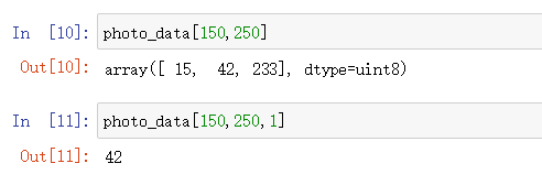
Pixel on the 150th Row and 250th Column

photo_data[150,250]

photo_data[150,250,1]

Set a Pixel to All Zeros

We can set all three layer in a pixel as once by assigning zero globally to that (row,column) pairing. However, setting one pixel to zero is not noticeable.

photo_revise = photo_data.copy()

photo_revise[150,250] = 0

fig,ax = plt.subplots(1,2,figsize=(20,10))
ax[0].imshow(photo_data),ax[1].imshow(photo_revise)

photo_revise = photo_data.copy()

photo_revise[150,250] = 0
photo_revise[200:800,:,:] = 255

fig,ax = plt.subplots(1,2,figsize=(20,10))
ax[0].imshow(photo_data),ax[1].imshow(photo_revise)

photo_revise = photo_data.copy()

photo_revise[150,250] = 0
photo_revise[200:800,:,:] = 0

fig,ax = plt.subplots(1,2,figsize=(20,10))
ax[0].imshow(photo_data),ax[1].imshow(photo_revise)

Changing Colors in a Range

We can also use a range to change the pixel values. As an example, let’s set the green layer for rows 200 to 800 to full intensity.

# set all three layers to full intensity


# set all three layers to 0

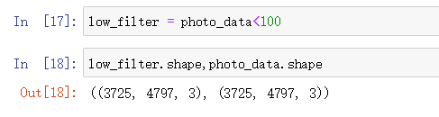
Pick all Pixels with Low Values

low_filter = photo_data<100

low_filter.shape,photo_data.shape

Filtering Out Low Values

Whenever the low_value_filter is True, set value to 0.

photo_revise = photo_data.copy()

low_filter = photo_data<200
photo_revise[low_filter]=0

fig,ax = plt.subplots(1,2,figsize=(20,10))
ax[0].imshow(photo_data),ax[1].imshow(photo_revise)

More Row and Column Operations

You can design complex pattens by making cols a function of rows or vice-versa. Here we try a linear relationship between rows and columns.

photo_revise = photo_data.copy()

length = len(photo_revise)

length

photo_revise[:length,:length]=0

fig,ax = plt.subplots(1,2,figsize=(20,10))
ax[0].imshow(photo_data),ax[1].imshow(photo_revise)

Masking Images

Now let us try something even cooler…a mask that is in shape of a circular disc.

photo_revise = photo_data.copy()

p_row,p_col,p_layer = photo_revise.shape

X,Y = np.ogrid[:p_row,:p_col]

X

Y

photo_revise.shape

c_row = p_row/2 
c_col = p_col/2
dist_c = (X-c_row)**2 + (Y-c_col)**2
r = (p_row/2)**2

mask = dist_c > r


print(mask[1200:1300,1200:1300])

photo_revise[mask] = 0

fig,ax = plt.subplots(1,2,figsize=(20,10))
ax[0].imshow(photo_data),ax[1].imshow(photo_revise)

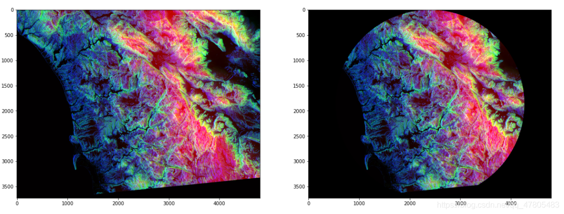
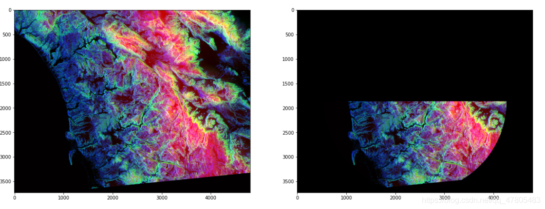
Further Masking

You can further improve the mask. For example, just get the upper half of the disc.

upper_half = X < c_row

mix_mask = upper_half | mask

photo_revise = photo_data.copy()

photo_revise[mix_mask] = 0

fig,ax = plt.subplots(1,2,figsize=(20,10))
ax[0].imshow(photo_data),ax[1].imshow(photo_revise)

Further Processing of our Satellite Imagery

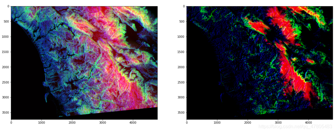
Processing of RED Pixels

Remember that red pixels tell us about the height. Let us try to highlight all the high altitude areas. We will do this by detecting high intensity RED Pixels and muting down other areas.

photo_revise = photo_data.copy()

mask = photo_revise[:,:,0] < 150
photo_revise[mask] = 0

fig,ax = plt.subplots(1,2,figsize=(20,10))
ax[0].imshow(photo_data),ax[1].imshow(photo_revise)

photo_revise = photo_data.copy()

mask = photo_revise[:,:,1] < 150
photo_revise[mask] = 0

fig,ax = plt.subplots(1,2,figsize=(20,10))
ax[0].imshow(photo_data),ax[1].imshow(photo_revise)

Detecting Highly-GREEN Pixels

photo_revise = photo_data.copy()

mask = photo_revise[:,:,2] < 150
photo_revise[mask] = 0

fig,ax = plt.subplots(1,2,figsize=(20,10))
ax[0].imshow(photo_data),ax[1].imshow(photo_revise)

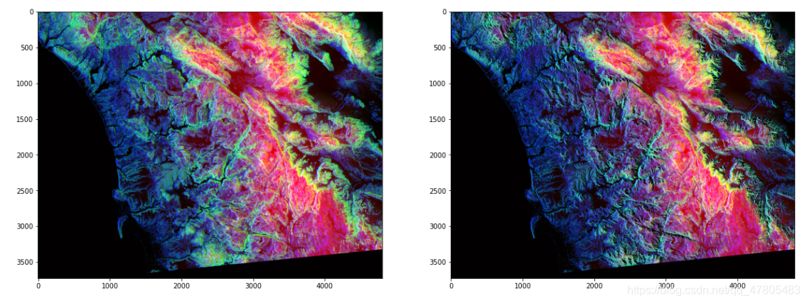
Composite mask that takes thresholds on all three layers: RED, GREEN, BLUE

photo_revise = photo_data.copy()

r_mask = photo_revise[:,:,0] < 150
g_mask = photo_revise[:,:,1] > 50
b_mask = photo_revise[:,:,2] < 100

photo_revise[r_mask|g_mask|b_mask] = 0

fig,ax = plt.subplots(1,2,figsize=(20,10))
ax[0].imshow(photo_data),ax[1].imshow(photo_revise)

photo_revise = photo_data.copy()

r_mask = photo_revise[:,:,0] < 150
g_mask = photo_revise[:,:,1] > 50
b_mask = photo_revise[:,:,2] < 100

photo_revise[r_mask&g_mask&b_mask] = 0

fig,ax = plt.subplots(1,2,figsize=(20,10))
ax[0].imshow(photo_data),ax[1].imshow(photo_revise)